This appendix explores the sensitivity of the baseline model forecast of the terms of trade to alternative assumptions.
Alternative metallurgical and thermal coal cost curves
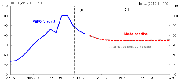
This sub-section explores the sensitivity of the terms of trade forecast to the use of alternative coal cost curve data sourced from Analyst-B, which have different coverage of both metallurgical and thermal coal seaborne production. These alternative coal cost curves were scaled using the methods described above, which produced virtually identical steel intermediate input and thermal coal supply curves. The resulting bulk commodity real unit value and export volume forecast based on these data are therefore very similar to those projected by the Wood Mackenzie data, which is reflected in the almost identical terms of trade forecast reported in Chart 32.
Chart 32: Terms of trade using alternative coal cost curve data
Source: Authors’ calculations.
Variation in the global demand for steel
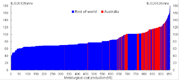
Cost curve data suggest Australian producers are situated around the middle of the iron ore cost curve and at the upper end of the metallurgical coal cost curve (Chart 33). Australian metallurgical coal export volumes are therefore expected to be sensitive to variations in the global demand for steel.
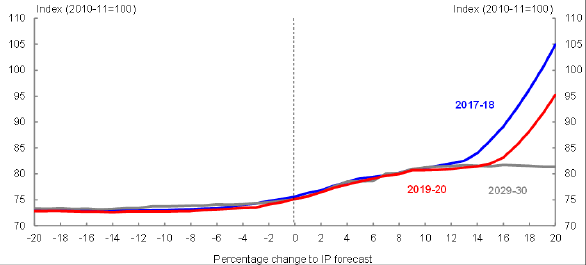
In this sub-section we explore the sensitivity of the terms of trade forecast to variation in industrial production (IP) which is the only exogenous input to steel demand. We test the sensitivity of the long-run terms of trade to variations in the global IP forecasts by varying the level of global IP over the projection period by a constant proportion ranging from -20 to +20 per cent.
Chart 33: Metallurgical coal cost curve (2013)
Source: Wood Mackenzie.
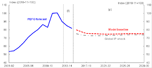
Chart 34 reveals that there are both price and volume effects associated with a change in steel demand. These effects are partially offsetting for both decreases and increases in IP. For example, a 10 per cent decrease in the forecast level of IP causes the projected iron ore price to be 25 per cent lower and the projected metallurgical coal price to be 11 per cent lower in 2019-20, while Australian exports volumes are projected to be 8 per cent lower for iron ore and 30 per cent lower for metallurgical coal. Since iron ore and metallurgical coal are the key commodities underlying the expected fall in the terms of trade and the prices of those commodities lie below all other relative prices, a decline in their export share partially offsets the fall in their relative price, leading to a terms of trade only 3 per cent lower in 2019-20 (Chart 35).
Chart 34: Sensitivity of long-run terms of trade forecasts to global IP forecast
Source: Authors’ calculations.
Chart 35: Terms of trade assuming 10 per cent weaker global IP
Source: Authors’ calculations.
Finally, it is important to emphasise that this analysis does not represent a comprehensive sensitivity analysis of the impact of a reduction in global IP on the terms of trade because a reduction in global IP would likely cause a decrease in the both the relative price and volume of all of the export categories, which would imply a greater fall in the terms of trade than reported here.
Comparison with other bulk commodity forecasters
In this sub-section we explore the sensitivity of the terms of trade forecast to alternative bulk commodity price and volume forecasts from BREE (2012 and 2013) and Consensus Economics (2013).
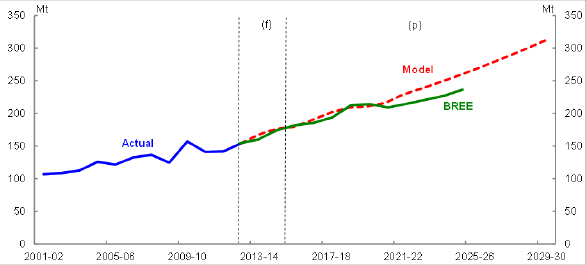
The effect on the terms of trade from using BREE’s price and volume forecasts of iron ore, metallurgical coal and thermal coal is shown in Charts 36 to 41. BREE (2013) provides price and volume forecasts until 2017-18. BREE volumes from 2018-19 are based on BREE (2013) 2017-18 forecasts and export growth rates implied by BREE (2012). In the case of iron ore and metallurgical coal we find that BREE’s volume forecasts are roughly similar to those generated by the global demand and supply models, while its real unit export prices lie above those generated by the global supply and demand model. In the case of thermal coal, BREE predicts much higher export volumes, but similar real unit export prices over the projection period. The resulting terms of trade profile from the BREE bulk commodity forecasts lies above that generated by the Treasury model (Chart 42).
One possible explanation for the differences between BREE’s and the Treasury’s bulk commodity forecasts is that BREE’s more detailed analysis incorporates freight costs, while the more stylised global demand and supply models employed here do not. Australian exporters are closer to Asian importing countries than many competitors, which suggests Australian exporters have a competitive advantage on freight costs. Preliminary analysis suggests that taking this geographic advantage into account would likely lead to slightly higher volumes and prices of Australian bulk exports than predicted by the global demand model.
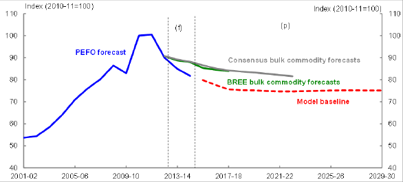
Next we consider the effect on the terms of trade of using the Consensus price forecasts for iron ore, metallurgical coal and thermal coal to 2022-23, which is the end of the Consensus forecast horizon (Charts 36, 38 and 40). Consensus does not provide volume forecasts so this sensitivity analysis uses the same volume forecasts as those presented above using the supply and demand framework. Consensus forecasts of bulk commodity prices lie above those generated by the steel and thermal coal demand and supply models, so it follows that the terms of trade profile generated using Consensus price forecasts is higher than the model based forecast (Chart 42). It is also the case that the Consensus profile is very similar to that derived from BREE bulk-commodity inputs up to 2017-18. Unlike the model based forecast, the Consensus profile suggests the terms of trade will continue to fall after 2017-18.
Chart 36: Australian iron ore real unit export price forecasts

Source: Authors’ calculations.
Chart 37: Australian iron ore export volume forecasts
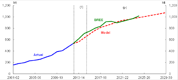
Chart 38: Australian metallurgical coal real unit export price forecasts
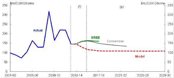
Chart 39: Australian metallurgical coal export volume forecasts
Source: Authors’ calculations.
Chart 40: Australian thermal coal real unit export price forecasts
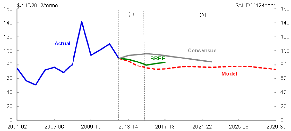
Chart 41: Australian thermal coal export volume forecasts
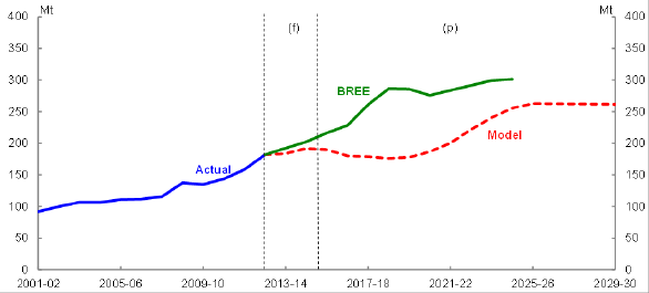
Chart 42: Terms of trade using external bulk commodity forecasts
Source: Authors’ calculations.
Non-rural non-bulk price forecasts
An analysis of the historical forecast accuracy of Consensus forecasts over the period from June 2005 to June 2013 finds a mean absolute percentage error of 28.9 per cent over a 10 quarter forecast horizon (there are not enough data to assess the accuracy of the Consensus long-run forecasts used for the terms of trade projection, but the accuracy of their 10 quarter ahead forecasts provides some guide to the accuracy of their longer-run forecasts). This high mean absolute percentage error reflects the difficulty in forecasting commodity prices, which are highly volatile.
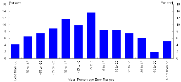
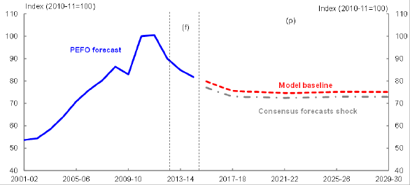
While Consensus forecasts have a high absolute percentage error, there is limited evidence of systematic bias in the direction of its errors. Overall, the mean percentage error for its forecasts of non-rural non-bulk commodities is -2.6 per cent over a 10 quarter forecast horizon, suggesting a slight conservative bias over the historical time period. Over a 10 quarter time horizon, Consensus forecasts on average overestimated the price of 5 commodities and underestimated the price of 5 commodities. Therefore, while Consensus forecasts have a high mean absolute percentage error, positive forecast errors for some commodities have tended to be offset by negative forecast errors for other commodities. This is demonstrated in Chart 43, which shows the distribution of quarterly consensus forecasting errors over a 10 quarter forecast horizon for the 10 commodities over the 6 year sample period 2005-2011 (creating 213 observations).
Chart 43: Distribution of Consensus forecasts mean percentage errors
Source: Authors’ calculations.
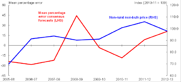
While there is little evidence of significant directional bias in Consensus forecasts over the entire sample period, since 2007-08 the Consensus forecasts have tended to overestimate prices over a period where prices have both risen and fallen, including over the last two years, when prices have been falling (Chart 44). This contrasts with the period from 2005-06 to 2007-08 over which Consensus forecasts tended to have a conservative bias over a period where prices were rising. It is likely that Consensus forecasts are slow to adapt to changes in prices, with Consensus forecasts remaining relatively high after a price fall and low after a price rise.
Based on the recent positive bias in Consensus price forecasts, we assess the effect on the terms of trade of Consensus forecasts for the non-rural non-bulk commodities that were systematically over-estimated by 20 per cent. Non-rural non-bulk commodities excluding LNG make up around 15 per cent of total export volumes. A 20 per cent reduction in the price of non-rural non-bulk commodities excluding LNG relative to import prices would therefore lead the terms of trade to be around 3 per cent lower (Chart 45).
Chart 44: Consensus mean percentage errors and non-rural non-bulk prices
Source: Authors’ calculations.
Chart 45: Terms of trade assuming weaker Consensus price forecast
Source: Authors’ calculations.
Exchange rate pass-through
The analysis to this point has assumed full pass-through of changes in the nominal exchange rate to import and export prices which implies no effect on the terms of trade from exchange rate fluctuations. While this assumption is true for rural goods export prices and non-rural commodities export prices, because they are almost entirely denominated in foreign currency terms, it need not be true for non-commodity goods and services because their prices depend on both domestic and foreign costs. In particular, domestic costs, especiall
y labour costs, are typically nominally sticky downward, so falling foreign costs are not typically matched by falling domestic costs. However, the reverse is likely to be the case, with higher foreign costs typically leading to higher domestic labour costs, and non-commodity goods and services prices.
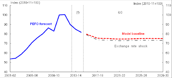
In light of Gruen and Wilkinson’s (1994) analysis of real exchange rates, Australia’s worsening terms of trade are expected to lead to a further depreciation of Australia’s real exchange rate over the projection period (beyond that assumed in the short-run 2013 PEFO forecast), which implies rising foreign input costs (i.e., higher import prices). Therefore, we test the sensitivity of the terms of trade forecast to the complete pass-through assumption by considering an extreme case of no pass-through of rising foreign input costs to domestic labour costs following a depreciation of the nominal exchange rate. This experiment should provide an upper bound on the responsiveness of the terms of trade to a depreciation of the exchange rate.
Chart 46: Terms of trade assuming lower nominal exchange rate
Source: Authors’ calculations.
The exchange rate is assumed to depreciate by 10 per cent relative to the level assumed in the baseline over the period from 2015-16 to 2017-18, which is consistent with the effect on the exchange rate of a 16 per cent fall in the terms of trade (i.e., the baseline model forecast) estimated by Gruen and Wilkinson. Under this scenario the long-run terms of trade are expected to be 2 per cent lower than the full pass-through model (Chart 46).