This section outlines the projection methodology for non-commodity goods and services export volumes and prices.
Analytical framework
Export volumes
Non-commodity goods and services exports are modeled by viewing them as imports of Australian goods by foreigners. Kouparitsas and Luo (2013) demonstrate that this approach leads to the following export demand equation:
![]() (3)
(3)
where at time t: Xit is the volume of Australian goods and services exports of category i; GNEFt is the trade-weighted index of foreign gross national expenditure (GNE) volumes; β1i is the elasticity of substitution between Australian and foreign produced varieties of goods and services category i; PXit is the Australian dollar price of Australian goods and services exports of category i; PGNEFt is the trade-weighted index of foreign GNE deflators; and TRENDt is a linear time trend that accounts for rising or falling foreign import penetration.
Export prices
We assume Australian firms have some power in the markets for Australia’s non-commodity goods and services exports, so the supply of these exports is modelled via a log-linear price mark-up equation, where the price of the export is a mark-up over nominal unit labour costs (i.e., total labour cost per unit of output) and possibly intermediate goods costs per unit of input. We further simplify this framework by assuming that there is no substitution between value-adding and intermediate goods and that all intermediate goods are imported (this is the form typically used in aggregate Australian price studies, such as De Brouwer and Ericsson, 1998), which implies the following log-linear export price equation:
![]() (4)
(4)
where at time t: WNULC t is the nominal unit labour cost; β1i is the share of total costs attributable to domestically sourced inputs; and TREND is a linear time trend.
This implies the following relative price relationship:
![]() (5)
(5)
Again, it is necessary to include a deterministic time trend to account for otherwise unexplained trends in the data, in this case the observed trends in the price of Australian export categories relative to economy-wide nominal unit labour costs and import prices. It is assumed that these trends will not continue in the long-run so they are held constant in the projection period.
Data
Historical annual exports data are sourced from the ABS Balance of Payments publication.
It is not possible to source GNE forecasts for many of Australia’s trading partners so more readily available foreign country GDP forecasts are used for all countries, in place of foreign country GNE. Detailed individual foreign country GDP historical data are sourced from various national statistical agencies and commercial data providers. Short-run forecasts of individual foreign country GDP from 2012-13 to 2014-15 are based on detailed bottom-up analysis consistent with the 2013 PEFO forecast, while forecasts from 2014-15 to end of the projection period are based on Au-Yeung, Kouparitsas, Luu and Sharma’s (2013) long-term projection methodology. Individual country GDP forecasts are weighted according to the respective country’s share of aggregate exports to form a trade-weighted foreign GDP forecast.
Forecasts of Australian nominal unit labour costs from 2013-14 to 2014-15 are based on Treasury’s 2013 PEFO forecast. Beyond 2014-15 nominal unit labour costs are assumed to grow at Treasury’s projection period expenditure price inflation assumption of 2.5 per cent.
Parameter estimation and calibration
The long-run export volumes and price equations are estimated using standard econometric techniques.
Non-commodity goods
It was necessary to introduce a level shift in 2008-09 (α1) to account for an otherwise unexplained fall in the level of non-commodity exports and a change to the coefficient of the deterministic trend in both 2000-01 (β3) and 2008-09 (β4) to account for an otherwise unexplained deceleration in the growth of non-commodity exports from 2000-01 to 2008-09 and 2008-09 to the end of the sample. The 2008-09 level and trend shifts coincide with the Global Financial Crisis (GFC).
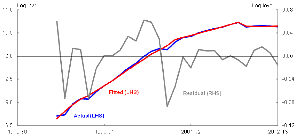
With an elasticity of substitution of 0.21 (β1), Australia’s non-commodity goods exports are gross complements, which implies the income effect associated with changes in the relative price of non-commodity exports dominates the substitution effect (Table 2). This is an important observation since it implies a modest response of exports volumes to changes in relative export prices. Chart 3 reveals the two slope shifts render the model’s residuals stationary.
Table 2: Non-commodity goods exports volume equation parameters
Method: Least Squares
Sample: 1984-85 2012-13
| Coefficient | Std. Error | t-Statistic | Prob. | |
|---|---|---|---|---|
| α0 | 7.865512 | 0.779031 | 10.09653 | 0.0000 |
| β1 | -0.206119 | 0.131440 | -1.568154 | 0.1305 |
| β2 | 0.065103 | 0.005486 | 11.86786 | 0.0000 |
| β3 | -0.053389 | 0.008146 | -6.553876 | 0.0000 |
| β4 | -0.041533 | 0.013406 | -3.098021 | 0.0051 |
| α1 | -0.110325 | 0.042553 | -2.592646 | 0.0163 |
| R-squared | 0.997009 | Mean dependent var | 10.00844 | |
| Adjusted R-squared | 0.996358 | S.D. dependent var | 0.667083 | |
| S.E. of regression | 0.040255 | Akaike info criterion | -3.405166 | |
| Sum squared resid | 0.037271 | Schwarz criterion | -3.122278 | |
| Log likelihood | 55.37491 | Hannan-Quinn criter. | -3.316569 | |
| F-statistic | 1533.219 | Durbin-Watson stat | 1.588499 | |
| Prob (F-statistic) | 0.000000 | |||
Source: Authors’ calculations.
Chart 3: Non-commodity goods export volume equation fitted values and residuals
Source: Authors’ calculations.
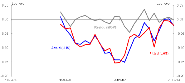
The estimated equation for non-commodity export prices is reported in Table 3. The coefficient on the imported intermediate goods variable (β1) implies roughly equal weight for domestic labour costs and imported intermediate goods in the determination of non-commodity goods export prices. The slope of the time trend (β2) is negative which suggests the non-commodity export sector displayed higher labour productivity growth than the aggregate economy over the estimation period. The residuals of this estimated equation are reported in Chart 4. They suggest the fitted equation captures the long-run trends of non-commodity export prices reasonably well as evidenced by the apparent stationarity of the residuals.
Table 3: Non-commodity goods export price equation parameters
Method: Least Squares
Sample: 1989-90 2012-13
| Coefficient | Std. Error | t-Statistic | Prob. | |
|---|---|---|---|---|
| α0 | -0.571642 | 0.046171 | -12.38104 | 0.0000 |
| β1 | 0.567991 | 0.051639 | 10.99937 | 0.0000 |
| β2 | -0.014709 | 0.001569 | -9.374137 | 0.0000 |
| R-squared | 0.859612 | Mean dependent var | -0.067914 | |
| Adjusted R-squared | 0.846242 | S.D. dependent var | 0.046793 | |
| S.E. of regression | 0.018348 | Akaike info criterion | -5.042071 | |
| Sum squared resid | 0.007070 | Schwarz criterion | -4.894814 | |
| Log likelihood | 63.50485 | Hannan-Quinn criter. | -5.003003 | |
| F-statistic | 64.29270 | Durbin-Watson stat | 1.485904 | |
| Prob(F-statistic) | 0.000000 | |||
Source: Authors’ calculations.
Chart 4: Non-commodity goods export price equation fitted values and residuals
Source: Authors’ calculations.
Services
The estimated equations for services volumes and prices are reported in Tables 4 and 5. Again, it was necessary to introduce level and growth rate shift terms to account for otherwise unexplained variation in volumes and prices at the time of the GFC. The services export volume equation is similar to the non-commodity goods equation, albeit with a higher elasticity of substitution of 0.56. Services export prices also place higher weight on nominal unit labour costs than non-commodity goods (i.e. 68 versus 57 per cent). In contrast to non-commodity goods exports, the positive coefficient on the time trend in the services exports price equation implies lower labour productivity growth than the aggregate economy over the estimation period.
Table 4: Services export volume equation parameters
Method: Least Squares
Sample: 1980 2013
| Coefficient | Std. Error | t-Statistic | Prob. | |
|---|---|---|---|---|
| α0 | 11.19148 | 0.471985 | 23.71152 | 0.0000 |
| β1 | -0.559259 | 0.098158 | -5.697537 | 0.0000 |
| β2 | 0.023799 | 0.001625 | 14.64382 | 0.0000 |
| β3 | -0.064630 | 0.019857 | -3.254730 | 0.0029 |
| α1 | -0.094221 | 0.053876 | -1.748851 | 0.0909 |
| R-squared | 0.991868 | Mean dependent var | 10.19533 | |
| Adjusted R-squared | 0.990746 | S.D. dependent var | 0.617073 | |
| S.E. of regression | 0.059362 | Akaike info criterion | -2.675285 | |
| Sum squared resid | 0.102190 | Schwarz criterion | -2.450820 | |
| Log likelihood | 50.47984 | Hannan-Quinn criter. | -2.598736 | |
| F-statistic | 884.2379 | Durbin-Watson stat | 0.642257 | |
| Prob(F-statistic) | 0.000000 | |||
Source: Authors’ calculations.
Table 5: Services export price equation parameters
Method: Least Squares
Sample: 1980–2013
| Coefficient | Std. Error | t-Statistic | Prob. | |
|---|---|---|---|---|
| α0 | -1.781096 | 0.055852 | -31.88936 | 0.0000 |
| β1 | 0.682936 | 0.048711 | 14.02029 | 0.0000 |
| β2 | 0.003659 | 0.001142 | 3.203714 | 0.0031 |
| R-squared | 0.982479 | Mean dependent var | -0.370650 | |
| Adjusted R-squared | 0.981348 | S.D. dependent var | 0.195022 | |
| S.E. of regression | 0.026634 | Akaike info criterion | -4.329123 | |
| Sum squared resid | 0.021991 | Schwarz criterion | -4.194445 | |
| Log likelihood | 76.59510 | Hannan-Quinn criter. | -4.283194 | |
| F-statistic | 869.1304 | Durbin-Watson stat | 0.635951 | |
| Prob(F-statistic) | 0.000000 | |||
Source: Authors’ calculations.
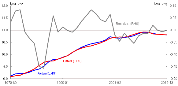
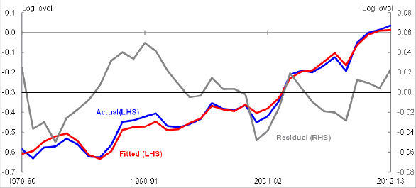
Plots of the services exp
ort volume and price equation residuals in Charts 5 and 6 suggest that the residuals are stationary.
Chart 5: Services export volume equation fitted values and residuals
Source: Authors’ calculations.
Chart 6: Services export price equation fitted values and residuals
Source: Authors’ calculations.
Forecasts
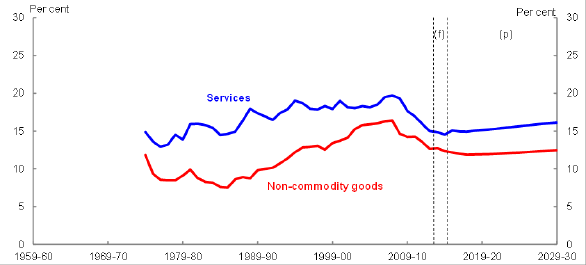
Chart 7 combines the short-run forecasts consistent with the 2013 PEFO and the long-run forecasts of the export volume models to generate a path for the volume shares of non-commodity goods and services over the projection period. The export volume shares of both non-commodity goods and services are expected to rise slightly over the projection period.
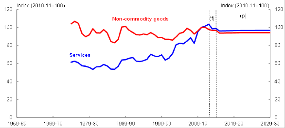
Similarly, Chart 8 combines the short-run forecasts consistent with the 2013 PEFO and the long-run forecasts of the export price models to generate a path for the relative prices of non-commodity goods and services over the projection period. Following a decline in non-commodity goods and services prices relative to imports over the forecast period, due in part to weak growth in nominal unit labour costs stemming from a weakening labour market, the long-run model implies constant relative prices over the projection period.
Chart 7: Export shares — non-commodity goods and services
Source: Authors’ calculations.
Chart 8: Relative export prices — non-commodity goods and services
Source: Authors’ calculations.