Blair Comley, Stephen Anthony and Ben Ferguson*
This article is devoted to examining the appropriate use of fiscal policy in the presence of private savings and interest rate offsets. The authors measure these effects in the Australian context and consider the implications of their empirical findings for the conduct of macroeconomic policy for a small open economy. This is an abridged version of a paper presented to the Bank of Italy Fiscal Policy Workshop in Perugia, Italy on 21 March 2002.
Background
Australian fiscal policy is based on a medium-term framework designed to ensure budget balance over the cycle. This medium-term framework ensures that the Government balance sheet remains in good order. The formulation of the fiscal strategy, with an `over the cycle' emphasis, also allows the use of fiscal policy as a demand management tool.
The fact that the strategy allows the use of discretionary fiscal policy raises the question of the desirability and effectiveness of discretionary fiscal policy. Australia is a relatively small, open, financially developed economy with a floating exchange rate. Standard economic theory suggests that monetary policy is a relatively more potent demand management tool for such economies. For example, it predicts that fiscal expansion will produce higher interest rates that will reduce investment expenditure. However, it also predicts that the instantaneous inflow of capital will to some extent circumvent any change in interest rates, and produce an appreciation of the currency and a smaller contribution of net exports to growth. In contrast, expansionary monetary policy leads to lower interest rates, capital outflow and a depreciated currency, which increases the net export contribution to growth. Symmetrically, with the first policy case, the capital outflow will mitigate the actual change in domestic interest rates.
From a policy maker's perspective it is important to have some understanding of the effectiveness of fiscal policy to inform the desirability and magnitude of any fiscal package. The paper does not attempt to ascertain the total effectiveness of fiscal policy. This paper focuses on two factors - private sector saving offsets and interest rate effects - that may reduce the effectiveness of fiscal policy as an aggregate demand management tool in Australia.
The paper is organised as follows. Section II considers evidence of private sector saving offsets in Australia. Section III considers the potential link between fiscal policy and interest margins. Section IV considers the policy implications of the paper's findings.
Fiscal policy and savings offsets
The following is a stylised description of the conventional view of the effects of a fiscal expansion where, for example, the government reduces taxes, with no planned reduction in current or future expenditures.
In the short run the effect of the government reducing taxes is to stimulate consumption which increases aggregate demand and in turn aggregate supply. This boost to consumption is partly offset in the short run by a range of crowding out effects - notably by higher interest rates reducing the level of investment and/or an appreciation of the exchange rate reducing net exports. In the long run the higher interest rate reduces capital accumulation and adversely affects growth. Notwithstanding these offsets and the long run effect on growth, fiscal policy does stimulate activity in the short-term. As such fiscal policy can be an effective tool for demand management.
However, another strand of literature that deals with Ricardian equivalence challenges this conventional wisdom (see Barro (1974)). Ricardian equivalence suggests that fiscal policy will not alter consumption, savings or growth.
Ricardian equivalence is based on the insight that lower taxes and a budget deficit today require, in the absence of any change in government spending, higher taxes in the future. If individuals are sufficiently forward-looking they will understand that their total expected tax burden is unchanged. As a result they will not increase consumption, but save the entire tax cut to meet their expected future tax liability. The decrease in government saving will thus be offset by an increase in private saving.
Perfect (or full) Ricardian equivalence relies on a very strict set of assumptions including: individuals' consumption choices fit a life cycle model of consumption; they are forward looking; and effectively `infinitely lived' through a bequest motive inspired by each generation's concern about the welfare of the next generation.1
The set of assumptions required for full Ricardian equivalence to hold is clearly unrealistic. However, the key issue for the effectiveness of fiscal policy is not necessarily whether all these assumptions hold, but rather whether there is some offsetting savings behaviour that may reduce the demand impact of fiscal policy. Furthermore, there are a range of other possible reasons that may illicit savings offsets at the appropriate level. For example, individuals may smooth their consumption or suffer from consumption inertia. This is essentially an empirical question. Our investigation of this empirical question is motivated by consideration of all these potential savings offsets.
International evidence suggests that an increase in public saving tends to lower private saving with an offset coefficient of around one half (Masson, Bayoumi and Samiei (1995); Callen and Thimann (1997); and Loyoza, Schmidt-Hebbel and Serven (2000)).
In contrast to these international studies, previous work with Australian data (Edey and Britten Jones (1990); Blundell-Wignall and Stevens (1992); and Lee (1999)) has found little evidence of Ricardian effects. But there are some issues with these studies which may have affected their findings. Blundell-Wignall and Stevens (1992) used annual data and regressed the change of the private saving ratio on the change of the public savings ratio. This approach, however, excluded other potential explanatory variables that may affect private savings (unemployment; income; inflation; and, real interest rate) potentially resulting in omitted variable bias and other specification problems. Lee (1999), used quarterly data and found no significant offset between household savings and changes in aggregate general government savings. Because there is no quarterly series available which directly measures private saving in Australia, a proxy must be used. However, it may have been preferable to use a broader measure of saving such as the household and corporate savings ratio as the relevant proxy.2
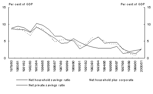
Chart 1 compares the annualised series for the quarterly household savings ratio and the household and corporate savings ratio to an annual measure of the private sector savings ratio. Chart 1 indicates that the household savings ratio in Australia is not the best proxy for overall private savings behaviour. The correlation coefficient between the private savings ratio and the household savings ratio over the period 1979-80 to 2000-01 is 0.83. In contrast, the household plus corporate savings ratio tracks the private sector savings ratio more closely, suggesting it is a better proxy for private savings. The correlation coefficient between the private savings ratio and the household plus corporate savings ratio over the period 1979-80 to 2000-01 is 0.91.
Chart 1: Comparison of net household, net household
plus corporate and private sector savings ratios
Source: ABS 56206-61; 5206-64; 5206-56; Treasury Estimates as per methodology outlined in Spring 1999 Economic Roundup, `The Measurement of Saving in Australia', pp
. 48-50.
We have investigated the potential link between the private savings ratio (net household plus corporate saving ratio) represented in Chart 1 and government savings over the period 1981:1 to 2001:2 (that is, March quarter 1981 to June quarter 2001). Our approach involved regressing the private saving ratio on a set of explanatory variables representing long-term fundamentals and short-term factors which tend to move the economy away from so called `equilibrium'.3
We hypothesise the long-term `equilibrium' level of private saving is a function of general government saving, controlling for the influence of the inflation rate, the unemployment rate, the real interest rate, per capita household disposable income, direct taxes, social assistance paid to households, household wealth, and household debt (a proxy for financial deregulation). In the short-term, changes in private saving are hypothesised to be a function of changes in general government saving, controlling for changes in the same set of `state' variables.
Private savings are anticipated to be negatively related to general government savings. This supposes that a fall in government saving would lead households to expect increased future tax liabilities and therefore to increase their saving rate in order to offset those expected future tax liabilities. Direct taxes and private wealth should be negatively related, while household disposable income should be positively related to private savings, both in levels and changes. A priori theory provides no unambiguous guide to the sign of the remaining variables.4
The model was initially run and insignificant variables systematically eliminated to produce the following model results reported in Table l.5
Table 1: Results from basic private savings model
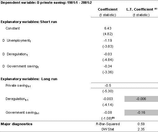
(a) The long-term coefficients in the table above are calculated by dividing the coefficients for the relevant variables by the coefficient on the error correction term (lagged value of the dependent variable).
(b) Redundant variable test for the inclusion of GSt-1: F statistic = 1.18 Prob = 0.281, Log Likelihood Ratio = 1.279 Prob = 0.258.
The above model suggests a significant private savings offset of around 1/3 to short-term changes in general government savings. In contrast to the short-term relationship, a long-term statistically significant relationship could not be established between the two variables at the 5 per cent confidence interval.
The model also suggests, that in the short run, the private savings ratio decreases by 1.2 per cent in response to a 1 percentage point increase in the unemployment rate, and falls by 0.03 per cent in response to a 1 per cent increase in household debt to disposable income ratio (the long run proxy for financial deregulation). The model suggests also that in the long run, a 1 per cent increase in the household debt to disposable income ratio elicits a 0.006 per cent decrease in the private savings ratio, so that there is evidence of a long term relationship between private savings and financial deregulation.6
Chart 2: Impulse response of private saving to a 1 per cent of GDP
permanent increase in government saving
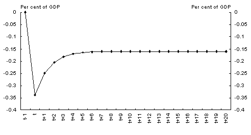
Chart 2 illustrates the impulse response for the level of private saving in response to a permanent 1 per cent of GDP increase in government saving. The chart demonstrates that it takes approximately 5 periods before the full effect of the shock is unwound and the system returns to it's long run equilibrium value of -0.16.
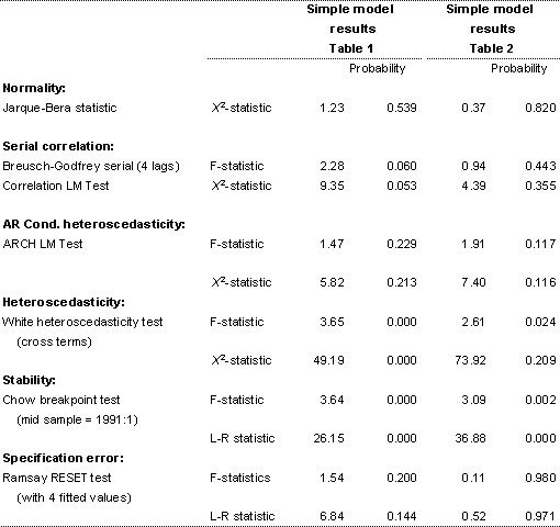
A complete summary of diagnostic tests are reported in Appendix 2. Based on these tests the model seems for the most part to have reliable characteristics. However, there is some evidence of autocorrelation and heteroscedasticity. Also, it is likely that the coefficient estimates are unstable over time and as such represent a major caveat on our results.
Another issue is whether private sector savings offsets are more pronounced in the face of `structural' rather than cyclical changes in government saving. Studies such as Cebula, Hung and Manage (1996) explore this proposition.
Cebula et. al. break the US federal budget into its structural and cyclical components. The former is hypothesised to be the `planned deficit', whereas the latter is viewed as the `unplanned'. They claim that the cyclical deficit can at best be crudely estimated, its determinants are sufficiently varied and unknown that predicting it is extremely difficult and beyond the capacities of most so called `rational' individuals. They argue that in a Ricardian world it is reasonable to expect that household saving will depend upon structural deficits, but cyclical deficits are likely to exercise little impact, if any, on household saving.7 They find for the US there is a private saving offset of around 1/3 on structural deficits, while cyclical deficits do not affect personal saving rates.
We have extended the model developed above by disaggregating general government saving into National general government structural and cyclical savings and State and Local general government savings.8
The model was initially run and insignificant variables systematically eliminated to produce the following model results reported in Table 2.9
Table 2: Results from disaggregated government model
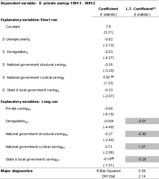
(a) The long-term coefficients in the table above are calculated by dividing the coefficients for the relevant variables by the coefficient on the error correction term (lagged value of the dependent variable).
(b) Redundant variable test for the inclusion of GSt-1: F statistic = 1.18 Prob = 0.281,
Log Likelihood Ratio = 1.279 Prob = 0.258.
The above model suggests that short-term increases in the National general government structural savings ratio of 1 per cent are partly offset by decreases in private sector savings of 0.35 per cent. Furthermore, the coefficient on the short-term changes in National general government cyclical savings term is not significant, suggesting that changes in this term do not elicit private sector savings responses. These results are consistent with the results reported above for the model incorporating an aggregate government saving measure.
However, in contrast to the earlier model, the disaggregated model also suggests a negative long-run relationship between National general government structural savings and private sector savings. A one per cent increase in the government structural savings ratio is associated with a 0.4 per cent decrease in the private savings ratio in the long-term.
While the model suggests a positive long-term relationship between cyclical government savings and private sector savings, we suspect that this relationship is largely due to cyclical factors affecting both terms rather than cyclical government savings provoking private sector responses. The long-term coefficient of 1.07 suggests that this is the case as both government cyclical savings and private savings seem to be affected one-for-one by cyclical factors. That said, we have estimated the equation with a range of cyclically sensitive variables, no
ne of which appear to be statistically significant. We would also note that cyclical government savings in the long-term are equal to zero. Therefore, any long-term effect between the two variables must be negated.
The model also suggests that changes in the unemployment rate and financial deregulation remain significant explanatory factors of private sector savings.
Chart 3: Impulse response of private saving to a 1 per cent of GDP
permanent increase in national government structural saving
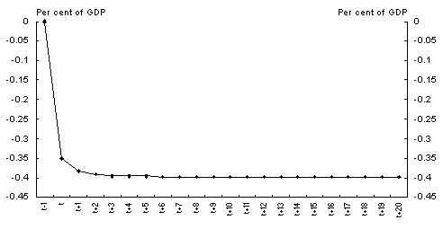
Chart 3 illustrates the impulse response for the level of private saving in response to a permanent 1 per cent of GDP increase in national government structural saving. The chart demonstrates that it takes approximately 3 periods before the full effect of the shock is realised as the system reaches it's long-run equilibrium value of -0.40.
A summary of standard diagnostic test statistics is reported in Appendix 2. Based on these the model passes the usual tests at standard significance levels, adjusted for heteroscedasticity. Once again, there is evidence that the coefficient estimates are unstable over time. However, given the relatively small sample we did not proceed with sub sample estimation.
These results suggest that the structural/cyclical decomposition is significant in terms of explaining private savings offsets. The previous model did not identify a statistically significant long-term equilibrium relationship between fiscal policy and private sector savings due to its focus on aggregate fiscal variables.10
The results of this model have interesting policy implications for the usefulness of fiscal policy as a demand management tool. Discretionary fiscal policy changes are (almost by definition) structural changes in government savings. Therefore, the results suggest that discretionary policy changes aimed at influencing aggregate demand are likely to be offset somewhat by private sector savings responses. This implies that any fiscal package needs to be larger than it otherwise would be in the absence of private sector savings offsets to have an effect on output.
However, in contrast to this, the operation of automatic stabilisers is unlikely to provoke private savings offsets as they represent cyclical changes in government savings. As a result automatic stabilisers may be seen as a more reliable option for managing demand than discretionary policy changes. That said, this needs to be qualified by the fact that there is scope to make the magnitude of discretionary policy changes substantially larger than the magnitude of automatic stabilisers. Furthermore, the results reported here necessarily refer to aggregate changes in savings behaviour. In principle certain individual fiscal measures may have much larger demand effects (for example, those that seek to change the timing of capital expenditure).
While the results from the above models have important implications for the effectiveness of fiscal policy, there is an important caveat.
It is possible that private saving is determined simultaneously with some explanatory variables in the regression equation. Explanatory variables that are likely to be endogenous with private savings include, government savings, and income growth. If such an endogeneity problem exists, the coefficient estimates of the model will be biased and inconsistent. While instrumental variables may be used to address this potential problem, finding persuasive instruments is difficult.
Fiscal policy and interest rates in Australia
The impact of fiscal policy on interest rates is important as the level of interest rates in Australia has significant short-term and long-term consequences. In general, higher interest rates will have adverse consequences for growth.
- If expansionary fiscal policy results in higher real interest rates, then this would operate to undermine short-term demand management by crowding-out to some extent the initial stimulus.
- Higher real interest rates can also lead to a lower long-term capital stock and a lower output level due to reduced investment levels. A lower capital stock and output level on average lowers living standards, real wages and employment levels (Elmendorf and Mankiw 1998, 28 and 29).
- Higher real interest rates also raise the long-term cost of servicing the stock of net foreign debt and thereby increase the level of transfers to foreign lenders (both public and private). It is possible that higher interest rates on debt also increase the cost of servicing foreign equity holdings. This is a particularly important issue for Australia given our relatively high level of net external liabilities (most of which have been incurred by the private sector).
There is little international evidence of a short-term link between fiscal policy and interest rates Ford and Laxton (1999, 80). Elmendorf (1996, 1) states that this may be due to the fact that the true relationship is between interest rates and the expected values of fiscal policy variables. Studies that have considered the link between interest differentials and expected fiscal policy, or 'risk premia' and expected fiscal policy, have found some evidence of a link to fiscal policy.11
More promising, pooled time series studies have suggested a link between interest differentials and actual fiscal policy. Orr, Edey and Kennedy (1995) show for seventeen developed countries between 1981:2 and 1992:2 that a 1 per cent of GDP fiscal stimulus increases the real interest rate differential on 10-year bonds by 15 basis points. Lane and Ferreti (2001) examined the OECD countries for the period 1970-98. Over this period they found a statistically significant relationship between public debt and the real interest differential (at the 10 per cent significance level).
For higher real interest rates to have significant economic effects they must operate at the long end of the yield curve by influencing society's preference (discount rate) for consumption over saving. Therefore, when considering the effect of interest rates on the economy it is important to focus on long-term bond rates which may be closer to the key determinants of long-term saving and investment decisions. This is not to say that short-term rates have no effect on saving and investment decisions. For example, home mortgage rates in Australia are closely tied to short-term interest rates.
In addressing the issue of the level of interest rates in Australia we focus on the return on Australian Commonwealth Government bonds. Of course Australian Government bonds may not be a perfect measure of the interest rate facing economic decision makers. However, we would expect that over reasonable periods of time arbitrage arrangements will result in the Government bond rate being a reasonable proxy for the level of interest rates facing economic agents. Chart 4 shows a relatively stable spread relationship between Australian Government and corporate bonds over the time period for which data is available. Analysing the government bond market also has the advantage that the market is highly liquid, reducing the risk of price discovery. Data are also readily available and collected on a consistent basis.
Chart 4: Spread between Australian government and
corporate bonds
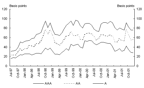
Source: RBA Bulletin, Table F.03m: Capital Market Yields and Spreads: Corporate Bonds: Monthly.
The interest rate on Australian Government bonds can be thought of as comprising of a nu
mber of components.
- First, if Australia is considered to be a small open economy there will be an infinitely elastic demand for Australian Government bonds. The interest coupon on these instruments can then be thought of as the base level of Australian interest rates given by the supply and demand for funds on the world market.
- Second, if we relax the assumption of an infinitely elastic demand then the interest rate may need to rise in order to attract additional investors. This effect can be thought of as the impact of the additional supply of bonds on the world market. This effect can be expected to be very small in the Australian context. Of course, if the same question were analysed for a country such as the United States, then this effect could be quite significant.
- Third, the above two possible determinants of Australian interest rates implicitly assume that all bonds are homogeneous. However, Australian bonds are likely to be viewed by investors as imperfect substitutes for other bonds. Investors may not be indifferent to the currency in which the bonds are denominated. Given that investors prefer to hold a balanced portfolio, they may require a higher return to increase the proportion of a particular country's assets in their portfolio, i.e. a portfolio risk premium (Frankel, 1979, 381).
- Fourth, investors may also demand a default premium to compensate for the probability that a country may default on its foreign debt obligations (Lonning, 2000, 262).12
- Fifth, if a country increases borrowing for purposes that do not increase the future supply of traded goods then a future depreciation will be expected to service the debt, which may lead to an interest differential now.
In this paper we focus on the margin on 10-year Treasury Bonds between Australia and the United States adjusted for expected inflation (see Data Appendix). The United States is used here as a proxy for the world market because it has historically been a major provider of capital to Australia and due to its role as a global safe haven. In terms of the taxonomy presented above, this methodology seeks to identify the combined effect of portfolio risk and default risk. The effect of Australian Government bond issuance on world interest rates (proxied here by the United States) will not be identified. Of course, other factors may affect the margin and so the estimates presented below need to be treated with caution.
This measured real interest margin calculated with expected prices is outlined for the period 1985:1 to 2001:2 in Chart 5. For purposes of comparison we have included a real interest margin measure constructed using actual prices as well.
Chart 5: The 10-year bond real interest margin between
Australia and the United States
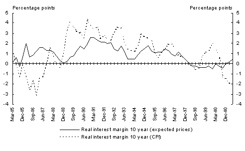
Source: Nominal interest rates and indexed bonds data obtained from RBA Bulletin and calculated as outlined in Appendix 1.
The high point of the `expected' margin was 257 basis points in December 1990 and the low point was -47 basis points in September 2000. In general, low values of the margin correspond to periods of fiscal consolidation in Australia (late 1980s and late 1990s) and high values during periods of fiscal expansion (early to mid 1990s).13 The following analysis seeks to explore this `observed' relationship more rigorously.
We have investigated the potential link between the real interest margin outlined in Chart 6 and actual fiscal policy over the period 1985:1 to 2001:2. Our approach is to attempt to explain movements in the interest margin over time by regressing it on a set of explanatory variables representing long-term fundamentals and short-term influences which tend to move the economy away from so called `equilibrium.14
We hypothesise a long-term `equilibrium' relationship where the level of the interest margin is a function of the levels of both the flow and stock of fiscal policy, controlling for `state' variables such as the inflation rate, real GDP growth rate, as well as the flow and stock of net foreign debt. Second, we hypothesise that short-term changes in the interest margin are a function of changes in the budget balance and stock of public debt, controlling for changes in the same set of `state' variables.
The interest margin is expected to rise in response to a deterioration in the budget balance or a rise in the stock of public debt. The interest margin is also hypothesised to be positively related to levels and changes in the inflation rate, and the stock of net foreign debt and negatively related to levels and changes in GDP growth and the current account.
The model was initially run and insignificant variables systematically eliminated to produce the following model results reported in Table 3, using the headline budget balance or structural budget balance, alternatively, as the fiscal flow variable.
Table 3: Interest margin model
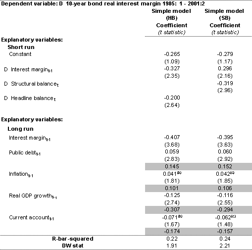
(a) The long-term coefficients for each equation are shaded grey and calculated by dividing the estimated coefficients for the relevant variables by the coefficient on the error correction term (lagged value of the dependent variable).
(b) Redundant variable test for the inclusion of Inflationt-1 and Current Accountt-1: F statistic = 3.83
Prob = 0.028 Log Likelihood Ratio = 8.31 Prob = 0.016.
(b) Redundant variable test for the inclusion of Inflationt-1 and Current Accountt-1: F statistic = 3.57
Prob = 0.036 Log Likelihood Ratio = 7.77 Prob = 0.020.
The model results reveal:
For the long-term levels component the fiscal stock variable (for example, stock of public debt) and real GDP growth were significant. The t statistic on the current account and inflation variable were not large enough to indicate a significant statistical relationship at the 5 per cent confidence interval. However, they are large enough to suggest there may exist a `meaningful' relationship between these variables and the interest margin.
For the short-term changes component, only the fiscal flow variables (for example headline balance or structural balance) were statistically significant.
The economic interpretation of the fiscal variables results in Table 3 is as follows. The interest margin increases by approximately 20 basis points in response to a one per cent of GDP deterioration in the headline budget balance. This is approximately the same magnitude of increase in the margin caused by a one percent of GDP increase in the stock of public debt at around 15 basis points. In contrast, a one percent of GDP deterioration in the structural budget increases the margin by approximately 32 basis points.
The economic interpretation of the `state' economic variables results in Table 3 is as follows. A one per cent of GDP increase in the current account deficit increases the margin by approximately 17 basis points in the long-term. A similar increase in the inflation rate increases the margin by approximately 10 basis points in the long-term. Importantly, a one-percentage point increase in the real GDP growth rate decreases the margin by approximately 31 basis points in the long-term.
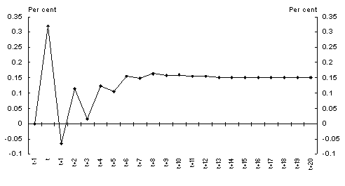
Table 3 reveals that the error correction term coefficient is around 0.40 for either version of the simple model and is statistically significant. The economic interpretation of this number is that the system reverts back to its long-term mean by 40 per cent in each quarter. Therefore it takes upwards of five quarters for short-term deviations from the long-term relationship to b
e unwound. This point is illustrated by examining the impulse response in Chart 6 which illustrates the adjustment path for the level of the interest margin after a temporary 1 per cent of GDP structural deterioration in the Commonwealth budget. The systems reverts to it's long-term value implying an increase in the interest margin of around 0.15 percentage points after approximately five quarters.
Chart 6: Impulse response of the interest margin to a 1 per cent of GDP temporary deterioration in the Commonwealth structural budget
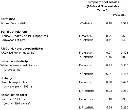
The model passes all the usual diagnostic tests at the standard significance levels as outlined in Appendix 2.
The implications for the conduct of fiscal policy stemming from these results are quite straightforward. Increases in the interest margin arising from public policy, for example default/portfolio risk, may reduce the effectiveness of fiscal policy to influence aggregate demand, and may have significant impacts on long-term growth and employment prospects.
Moreover, it seems likely from these results that changes in the structural budget (for example, discretionary spending) drive short-term changes in the interest margin. This implies that significant discretionary fiscal policy movements may have large associated costs.
Finally, we would note that the magnitudes of the fiscal coefficients estimated previously are quite large given that Australia is a small open economy, although they are consistent with the international literature examined previously. As such we would not want to over-play the significance of the magnitudes presented here.
For completeness we note that there are some important provisos that must be placed on the numbers described previously.
The results may suffer from endogeneity problems given budget deficits, income and interest rates may be determined simultaneously.
There is no role of information and expectations in the simple model which is unorthodox given that we are attempting to explain the interest margin between two financial assets.
Conclusion
The paper considers the effectiveness of fiscal policy with respect to two key issues: potential private sector savings offsets; and the link between fiscal policy and interest rates in Australia. These two issues are important when considering the role of fiscal policy in Australia. Evidence of significant private sector savings offsets would indicate that fiscal policy is less effective as a demand management tool than it otherwise would be. Evidence of increasing interest rates in response to higher budget deficits would indicate that fiscal policy is less effective as a demand management tool and that there may be adverse consequences for long-term living standards.
Previous Australian studies have found little evidence of substantial private savings offsets. In contrast, our results indicate the existence of a substantial private savings offset. We investigate the relationship between private and public savings in two ways. First, we estimate a model that focuses on aggregate government savings. The results of this model suggest that there is a private savings offset of around one third in the short run. The results from this model do not support the existence of a long run relationship between private and government savings. Second, we estimate a model that disaggregates government savings into structural and cyclical components. The disaggregated model suggests a similar short-term private savings offset of around one third. However, the disaggregated model provides two additional insights. First, the disaggregated model suggests that the short run private savings offset is associated with changes in structural government savings, but that there is no statistically significant relationship between private savings and cyclical government savings. Second, the disaggregated model suggests that there is a long run private savings offset of around a third to changes in structural government saving.
There are two key implications of these results. First, the magnitude of any fiscal stimulus will need to be larger than it would otherwise need to be in the absence of savings offsets to have the same effect on aggregate demand. Second, the operation of automatic stabilisers (which are inherently changes in cyclical government saving) are likely to be relatively more effective than discretionary changes in policy (which are inherently changes in structural government saving). This last point needs to be qualified by the observation that our results are based on aggregate data and therefore may not capture the demand effects of specific policies that may in practice have more potent demand effects.
The paper also considers the link between fiscal policy and interest rates in Australia. We estimate a model that seeks to explain variations in the 10-year bond real interest margin with the United States with reference to variables including the headline budget balance, and the level of net public debt. The results suggest that a deterioration of the headline balance of one per cent of GDP is associated with an increase in the margin of around 20 basis points in the short run and that an increase in public debt of one per cent of GDP is associated with an increase in the margin of around 15 basis points in the long run. Furthermore, when we re-estimate the model using the structural balance instead of the headline balance, we find that the effect of changes in the structural balance on the margin is even higher at around 30 basis points.
These results suggest that higher budget deficits (or lower surpluses) can have a significant effect on interest rates in Australia. The associated costs of higher interest rates should be borne in mind when setting fiscal policy. That said, the size of the interest rate changes suggested by these results appear very high for a small economy with access to international financial markets such as Australia. Accordingly, we believe that these results should be treated with some caution. These coefficients belong to an era of higher debt. We would be surprised if further debt reduction had as large an incremental effect in this era of low debt.
Bibliography
Savings offsets
Banca D'Italia, (1999), `Indicators of structural budget balances', Research Department Public Finance Workshop, Perugia, 26-28 November 1998.
Barro, R. (1974), `Are Government bonds net wealth?', Journal of Political Economy, Vol. 82, pp. 1095-1117.
Blundell-Wignall, A. and Stevens, G. (1992), `Fiscal policy in Australia: Recent developments and current issues', Current Issues in Fiscal Policy and Their Implications for the Conduct of Monetary Policy, Bank for International Settlements, pp. 1-31.
Callen, T. and Thimann, C. (1997), `Empirical determinants of household saving: Evidence from OECD countries', International Monetary Fund, Working Paper, WP/97/181.
Cebula, R.J., Hung, C.S. and Manage, N.D. (1996), `Ricardian equivalence, budget deficits, and savings in the United States', Applied Economics Letters, Vol. 3, pp. 525-528.
Commonwealth Treasury (1999), `The measurement of saving in Australia,' Economic Roundup, Spring, pp. 21-51.
Edey, M. and Britten-Jones, M. (1990), `Saving and investment', The Australian Macro-Economy in the 1980s, Reserve Bank of Australia, pp. 79-145.
Elmendorf, D. and Mankiw, N. (1998), `Government debt', National Bureau of Economic Research, Working Paper, No. 6470.
Engle, R. F. and Granger, C.W.J. (1987), `Co-integration and error correction: representation, estimating and testing', Econometrica, Vol 55, pp. 251-276.
EVIEWS 3.1, (1998), Quantitative Micro Software, Irvine California.
Giorno, C., Richardson, P., Roseveare, D. and van den Noord, P. (1995), `Potential output, output gaps and structural budget balances', OECD Economic Studies, No. 24. pp. 167-209.
Hendry, D. A. (1995) Dynamic Economics, Oxford, Oxford University Press.
Lee, J. (1999), `Australia: household saving', International Monetary Fund, Australia: Selected Issues and Statistic Appendix, pp. 36-43.
Loyoza, N., Schmidt-Hebbel, K. and Serven, L. (2000), `What drives saving across the world?', Review of Economics and Statistics, Vol. 82, pp. 226-238.
Masson, P., Bayoumi, T. and Samiei, H. (1995), `International evidence on the determinants of private saving', World Bank Economic Review, Vol. 12.
Interest margin
Elmendorf, D. W. (1993), `Actual budget deficits expectations and interest rates', Harvard Institute of Economic Research, Discussion Paper Series, No. 1639, May.
Elmendorf, D. W. (1996), `The effects of deficit-reduction laws on real interest rates', Finance and Economics Discussion Series, Federal Reserve Board, Divisions of Research and Statistics and Monetary Affairs, 44.
Elmendorf, D. W. and Mankiw, G. N. (1998), `Government debt', National Bureau of Economic Research, Working Paper, No. 6470, March.
Engle, R. F. and Granger, C.W.J. (1987), `Co-integration and error correction: representation, estimating and testing', Econometrica, Vol. 55, pp. 251-276.
EVIEWS 3.1, (1998), Quantitative Micro Software, Irvine California.
Frankel, J. A. (1979), `The diversifiability of exchange risk', Journal of International Economics, 9, pp. 379-393.
Ford, R. and Laxton, D. (1999), `World public debt and real interest rates', Oxford Economic Review of Economic Policy, Vol. 15, No. 2, pp. 77-94.
Giorgianni, L. (1997), `Foreign exchange risk premium: Does fiscal policy matter?' Evidence from Italian data', International Monetary Fund, Working Paper, No. 39, March.
Lane, P. R. and Milesi - Ferretti, G.M. (2001), `Long-term capital movements', National Bureau of Economic Research, Working Paper , No. 8366, July.
Lonning, I. M. (2000), `Default premia on European government debt', Review of World Economics, Vol. 136, No. 2, pp. 259-283.
Orr, A., Edey, M. and Kennedy, M. (1995), `The determinants of real long-term interests rates: 17 country pooled-time series evidence', OECD Economics Department, Working Paper, No. 155.
Appendix 1: Data
Savings offsets
Ratio of net household plus corporate saving to GDP. Net household savings (ABS 5206-61); Net corporate savings calculated as the residual of net national savings minus net household savings and net general government savings; GDP (ABS 5206-56).
Household disposable income per capita. Nominal Household Disposable Income (ABS 5206-61); CPI (RBA Bulletin Table G.01); Population (ABS 3101-04).
Unemployment rate (ABS 6202-04).
Inflation rate (RBA Bulletin Table G.01).
Real interest rate. Interest Rate (10 year Treasury bond yield (RBA Bulletin Table F.02)); Inflation (RBA Bulletin Table G.01).
Net General Government Savings to GDP ratio (ABS 5206-64)
Net Commonwealth General Government Structural Savings to GDP ratio.
Net Commonwealth General Government Cyclical Saving to GDP ratio.
Net State and Local General Government Savings to GDP ratio (ABS 5206-66).
Share of Commonwealth indirect taxes to total Commonwealth General Government taxation revenue (RBA Bulletin Table E.01m).
Social assistance benefits to household disposable income ratio (ABS 5206-61).
Household debt to household disposable income ratio (RBA Bulletin Table D.02).
Private wealth to household disposable income ratio (ABS TRYM Database Table 33).
All components were seasonally adjusted using X11 in EVIEWS.
Interest margin
10-Year Bond (RBA Bulletin Table F.02d).
Expected Inflation - nominal 10-year bond yields and inflation indexed bond yields - (RBA Bulletin Table F.02d)
Federal General Government Headline Balance (RBA Bulletin Table E.01m) seasonally adjusted using the X11 divided by annualised level of GDP, (OECD Main Economic Indicators Table Aus.01).
Federal General Government Structural Balance obtained from Fiscal Policy Unit of the Australian Treasury - divided by annualised level of GDP, (OECD Main Economic Indicators Table Aus.01).
Net Public Sector Debt (ABS Table 5302.35) divided by annualised level of GDP, (OECD Main Economic Indicators Table Aus.01).
Inflation ABS (Table 6401.011). The CPI measure includes all groups excluding housing.
Real GDP Growth (OECD Main Economic Indicators Table Aus.01)
Current Account (Table 5302-04) and GDP (Table 5206-22) data were obtained from the ABS. Both series were seasonally adjusted.
Net Foreign Debt ABS (Table 5302.35), not seasonally adjusted, in current prices. Divided by annualised level of GDP, (OECD Main Economic Indicators Table Aus.01).
Appendix 2: Diagnostics
Savings offsets parsimonious models
Interest margin
1 For a full set of assumptions underpinning Ricardian equivalence see Elmendorf and Mankiw (1998).
2 One reason for this may be the long-term trend in Australia towards the incorporation of non-incorporated businesses.
3 We employed the Johansen-Julieus ECM approach for modelling with non-stationary variables. We recognise that while there may exist a long run equilibrium relationship between the variables under examination, there may be disequilibrium in the short-term. The framework, therefore, models the change in the dependant variable as a function of changes in the explanatory variables and the error correction mechanism, in which a proportion of the disequilibrium in one period is corrected in the next.
4 Unemployment: Increasing unemployment lowers disposable income and, through a greater incidence of liquidity constraints, lowers savings. On the other hand, increases in unemployment may increase the need for precautionary saving.
Inflation: Inflation tends to undermine the value of financial assets and stimulate saving. On the other hand, it may also reduce the return from saving in financial rather than non-financial assets, which tends to lower saving.
Real interest rates: The sign of the effect depends on whether the substitution or income effect dominates.
Deregulation: Financial deregulation may increase the opportunities for, and return to, financial savings, but may also enhance access to credit and thus lower private savings.
5 For unit root tests, tests for joint significance and full model results please refer to the conference edition of this article. All estimation and diagnostic procedures undertaken for the purposes of this paper were performed in EVIEWS 3.1.
6 While the coefficients on the financial deregulation terms are low, financial deregulation does seem to have a significant effect on private savings as the household debt to disposable income ratio is a very high value.
7 This point was also made by Barro, (Edey and Britten-Jones, 1990, pp. 120-121), who noted that both public and pri
vate savings tend to move cyclically, and in order to determine the effect of public sector deficits on private saving, the exogenous component of the public sector position must first be extracted. An alternative explanation is that cyclical deficits do not require a future increase in the tax rate, as higher tax revenue is automatically generated, so there is no need for anyone to increase their savings rate.
8 We note that determination of the structural and cyclical components of savings involves a range of complex issues (see Banca D'Italia, 1999). However, while the level of structural savings is particularly difficult to identify it is more straightforward to determine changes in structural savings. The changes in structural savings are of primary importance in generating the results contained in this paper.
9 We have not broken the State and Local Government savings numbers down into structural and cyclical components due to the lack of quarterly data available to conduct the analysis. It is likely that variations in State and Local Government savings positions are primarily structural in nature due to the heavy revenue reliance on the Commonwealth and the fact that State and Local Government outlays are less cyclically sensitive than Commonwealth outlays reflecting the Commonwealth's primary responsibility for income support arrangements. Furthermore, separately identifying the State and Local Government sector is useful as it allows us to focus on the savings behaviour of the Commonwealth Government which in practice is responsible for demand management policy.
10 This factor may also help to explain the results of Lee (1999), where, in addition to using the household savings ratio as the dependant variable, the study used cointegration analysis on the levels of the household savings and actual general government savings ratios.
11 For example Elmendorf (1993), Elmendorf (1996) and Giorgianni (1997).
12 Conceptually the default risk premium is a subset of portfolio risk. It is one of the reasons why investors do not view all government bonds as perfect substitutes. That said, we believe that it is useful to identify it separately as the risk of default is a common focus when sovereign debt issues are considered. Separately identifying default risk highlights the fact that investors may believe that there is a zero default risk, but still demand higher returns to hold a higher proportion of a particular countries' bonds. This is important for a country like Australia where default risk is likely to be perceived by investors as close to zero.
13 Of course there is an issue of observational equivalence here because in times of high growth a government has more capacity to eliminate debt which will assist in driving down yields, and vice versa in periods of recession.
14 Details of all data sources used for this study are contained in Appendix 1.
