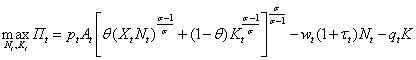
Lewis and MacDonald (2002) and a host of others have demonstrated that long-run aggregate demand for labour in Australia is well-approximated by the first order condition for labour derived by solving a standard profit maximisation problem of a representative firm subject to a constant elasticity of substitution (CES) production function. The representative firm's profit maximisation problem can be presented as follows:
![]() (1)
(1)
subject to a constant returns to scale and CES production function:
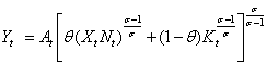 (2)
(2)
where: ∏t is profit at time t; pt is output prices; Yt is output (volume); wt is nominal wages; ![]() is the payroll tax rate; Nt is employment; qt is the rental rate of capital; Kt is capital; At is Hicks-neutral technical change; 0 < θ < 1 is a weighting parameter; Xt is labour-augmenting technical change (Harrod-neutral); and σ > 0 is the elasticity of substitution between capital and labour.
is the payroll tax rate; Nt is employment; qt is the rental rate of capital; Kt is capital; At is Hicks-neutral technical change; 0 < θ < 1 is a weighting parameter; Xt is labour-augmenting technical change (Harrod-neutral); and σ > 0 is the elasticity of substitution between capital and labour.
For ease of exposition and without loss of generality, we assume that the firm's production function is always binding, which allows us to solve the following problem:
 (3)
(3)
The resulting necessary first order condition for labour  implies:
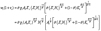 (4)
(4)
Substituting (2) into (4):
![]() (5)
(5)
and solving for labour (Nt) implies:
![]() (6)
(6)
Taking logarithms gives the following labour demand relationship, conditional on the level of output, labour-augmenting technical change and real wages:
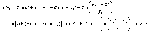 (7)
(7)
This expression can be simplified further by noting that there are no cyclical fluctuations over the long-run, so in the long-run At will be at its average level A, which yields the following long-run labour demand equation:
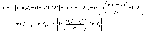 (8)
(8)
where: ![]()
Equation (8) gives the logarithm of long-run labour demand as equal to three terms: a constant, the logarithm of real output adjusted for labour-augmenting technical change, and the elasticity of substitution multiplied by the logarithm of the real wage adjusted for labour-augmenting technical change (that is, the logarithm of long-run real unit labour costs). The effect of an increase in the level of labour-augmenting technical change on labour demand depends on the size of the elasticity of substitution between capital and labour: other things equal, labour demand decreases if σ < 1 and increases if σ > 1.