3.1 Data source and sample
Data are drawn from waves five, six, and seven of the `in-confidence' version of the Household, Income and Labour Dynamics in Australia (HILDA) Survey which cover the period 2005 - 2007. The HILDA Survey is an annual panel survey of Australian households which was begun in 2001.7 There are approximately 7,000 households and 13,000 individuals who respond in each wave. The choice of data is based upon four considerations.
Firstly, and most importantly, the HILDA survey data from wave five onwards collected child care usage data separately by child. It also collected data on hours of child care used to support paid employment and hours of child care used for other reasons such as freeing up time for mothers or for educational reasons. In the first four waves, data was more aggregated within the household.
Secondly, we choose to pool across three waves of data to achieve a sufficiently large sample size. This is important in the construction of our local average child care price, described in detail in section 3.2 below.
Thirdly, there were no major changes to the Child Care Benefit (CCB) scheme during this period. One potential complication, however, is the introduction of the Child Care Tax Rebate (CCTR), now called Child Care Rebate (CCR), which was announced at the beginning of our sample period. In its initial form, this rebate was paid with a two-year lag after child care expenses were incurred and its coverage was limited; being only available as an offset against tax paid. Even though access to the rebate was eased from July 2007, with the two-year lag reduced to one year and the rebate extended to non-taxpayers, it remains the case that over the period of the estimation data there was a considerable lag between the incurring of child care expenses and the receipt of any rebate.
We decided not to include the rebate in constructing the child care price variable and to not include CCTR in construction of our model. The decision to not include the rebate in the price is supported by comparing the 2005-07 data on net child care expenses reported by households in our survey data to average prices from administrative data. The best match to the administrative data is generated by assuming that respondents take account of CCB, but not the rebate, in their calculation of net child care expenses. The decision to not include CCTR in construction of our model is because it would not have recognised the lag at the time between the decision to use child care and payment which would be expected to have weakened the incentive effect of the rebate and diluted the labour supply response. The suggestion is that people at that time would have only partly, if at all, factored an entitlement to the rebate (payable at some time in the future) into their child care and labour supply decisions.
Ignoring CCTR in our model estimation does not mean that we think that there were no labour supply effects of CCTR at that time. Rather, it is our judgment that it is more realistic to assume that the rebate had no impact, than to assume that it had full impact. The truth, of course, will lie somewhere between these extremes, though in our view it is likely to have been closer to the no impact assumption.
The complexity of the model and the non-linearity of the budget constraint make it impossible to say with confidence the way in which this might bias our results. Our intuition is that ignoring the rebate may lead us to somewhat overstate the labour supply responses, particularly for higher-income households. Any effect is likely to be small.
This exclusion of CCTR from the model estimation does not limit the ability or the appropriateness of the model for analysing policies such as the current CCR. There are two reasons for this. First, since the model is estimating underlying parameters of the utility function which are not dependent on the specific policy settings which are in place during the sample period, the model is still valid for studying any personal tax and transfer policy related to child care and labour supply including rebates. Second, CCR nowadays is quite different from its initial CCTR form. Since the period of the estimation data (2005 to 2007), the rebate has been increased from 30 to 50 per cent of out-of-pocket expenses, the maximum value of the rebate has been increased substantially, and the lag between the incurring of expenses and payment of the rebate has been further reduced. CCR in its current form would be expected to have a far stronger impact on child care and labour supply decisions than did its predecessor.
A final consideration which favours this choice of sample period is that the Australian Bureau of Statistics (2010) created a gross child care price index from 2005, which we use to make the price comparable across waves.8
We focus on the labour supply of partnered mothers with at least one pre-school child and the demand for formal child care in these households. In waves 5 through 7 of the HILDA survey there are 20,342 observations on 7,741 women. Once we remove women from the sample who are neither married nor in defacto relationships, there are 12,109 observations on 4,754 women. Excluding those families with no pre-school children further reduces the sample to 2,601 observations on 1,198 women. Pre-school children are defined as children age five and under who are not attending school. We exclude a further 131 observations on 92 women who live in multiple-family households and 219 observations on 156 women who are studying full-time. This leaves us with an estimation sample of 2,251 observations on 1,069 women across the three waves. After discarding observations with missing values for any variables used in our model (excepting wage), the sample consists of 2,023 observations on 978 partnered mothers with at least one pre-school child.
Note that households with school-aged children, but without pre-school children, are omitted from our analysis sample. Our rationale for this is that the labour supply and child care issues faced by those households may be quite different from those with pre-school children. Importantly, school-aged children attend school for around 30 hours per week, which makes their need for maternal or non-maternal child care much less than that of younger children. This sample of households with pre-school children, for these reasons, will be a more homogeneous sample which should reduce the influence of unobserved preferences on observed outcomes. This sample homogeneity allows for a simpler model and provides a reduction in bias.
We present sample statistics in the second column of Table 1. In the third column of Table 1 we present the sample statistics for a sub-sample of 1,159 mothers of pre-school children in households in which there are no school-aged children present. This sub-sample is used for sensitivity analysis as described below. From the second column of Table 1, about 43 per cent of households with pre-school children use formal child care. Hours spent in child care for the pre-school children are about 18 hours per week. About 56 per cent of the mothers were employed and the average working mother works 25 hours per week at an hourly wage of $25 (at the June 2005 price level). The characteristics of the mothers in the sub-sample are broadly similar to those of the whole sample except they are younger and slightly better educated.
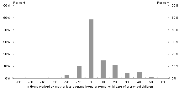
Many households use less formal child care than the mother's hours of work. To see how mothers' working hours and formal child care hours are related, Figure 3 presents the distribution of the difference between the two. Figure 3 shows that in about more than thirty per cent of households with pre-school children, the average reported hours of formal child care per pre-school child are less than the mothers' reported hours of work. This indicates that the quantity cons
traint (that formal child care hours are greater than or equal to hours worked by the mother) imposed by Duncan et al. (2001) and Kornstad and Thoresen (2007) is probably too restrictive.
| Variables | Partnered mothers with at least one pre-school child | Partnered mothers with pre-school children but with no school-aged children |
|---|---|---|
| Hours worked per week (for those mothers who are working) | 24.8 (13.7) | 25.6 (13.5) |
| Employment rate (mothers) | 0.56 | 0.60 |
| Average hours of formal child care (per child) for children using formal care | 18.8 (12.9) | 19.0 (13.2) |
| Proportion of families using formal care | 0.43 | 0.45 |
| Hourly wage rate of the mother (at June 2005 price) | 25.3 (22.5) | 26.6 (22.1) |
| Weekly household income from father's earnings and unearned private income | 1238 (1242) | 1305 (1289) |
| Median hourly child care price (at June 2005 price) | 4.67 (0.92) | 4.73 (0.98) |
| Age of the mother | 32.9 (5.9) | 31.8 (5.8) |
| Dummy variables for highest level of education received: | ||
| Mother received higher education | 0.34 | 0.41 |
| Mother received vocational education | 0.25 | 0.24 |
| Mother finished Year 12 only | 0.21 | 0.21 |
| Mother did not finish Year 12 | 0.21 | 0.14 |
| Father received higher education | 0.27 | 0.30 |
| Father received vocational education | 0.42 | 0.40 |
| Father finished Year 12 only | 0.14 | 0.16 |
| Father did not finish Year 12 | 0.17 | 0.14 |
| Dummy, mother did not live with both parents at the age of 14 | 0.22 | 0.22 |
| Dummy, equals one if the mother was not born in Australia, but was educated in Australia | 0.14 | 0.15 |
| Dummy, equals one if the mother was educated and born outside of Australia | 0.05 | 0.06 |
| Dummy, the mother speaks a language other than English | 0.12 | 0.11 |
| Dummy, the mother is Aboriginal or and Torres Strait Islander | 0.02 | 0.02 |
| Dummy, equals one if mother and the father both educated in Australia and both born outside of Australia. | 0.19 | 0.20 |
| Dummy, equals one the mother and the father are both born and educated outside of Australia | 0.10 | 0.08 |
| Number of children aged 0 to 4 | 1.3 (0.6) | 1.4 (0.6) |
| Number of children aged 5 to 12 | .60 (0.8) | - |
| Number of children aged 13 to 15 | .09 (0.3) | 0.05 (0.25) |
| Age of the youngest child | 1.5(1.5) | 1.1 (1.2) |
| Dummy, presence of female adult in the household other than the mother | 0.03 | 0.03 |
| Dummy, presence of children older than 12 in the household | 0.87 | 0.78 |
| Mean age of children | 1.9 (1.4) | 1.5 (1.2) |
| Dummy variables equal to one if current state of residence is: | ||
| NSW | 0.28 | 0.27 |
| VIC | 0.25 | 0.26 |
| SA | 0.08 | 0.07 |
| WA | 0.10 | 0.11 |
| TAS | 0.03 | 0.02 |
| NT | 0.01 | 0.01 |
| ACT | 0.03 | 0.03 |
| % of child care staff with teaching experience (state average) | 15.7% (4.4%) | 15.7% (4.4%) |
| % of child care staff with teaching qualification (state average) | 66.9% (5.0%) | 66.9% (5.0%) |
| Observations (number of partnered mothers) | 2,023 | 1,159 |
Note: Standard deviations are in the parentheses.
Figure 3 Hours worked by mothers less average formal child care hours of pre-school children
3.2 Child care price
Gong et al. (2010) show that measurement error in the child care price can have large effects on results in labour supply and child care demand models. In this paper, we follow their method to construct the child care price. The model is designed to evaluate how families respond to changes in child care price in terms of their demand for child care and mothers' labour supply. We thus need a price that reflects a `typical' amount that a household will have to pay if they choose to increase hours of formal child care (or an amount they will save if they decrease formal hours of child care).
There are two problems that arise. The first is that we need a child care price that applies to families who are not currently using any child care. As price changes, these families may begin to use child care and we need a price to evaluate this possibility.
When families purchase child care they are purchasing a bundle of attributes. They are paying the cost of having their children cared for at some basic standard. But t
hey are also paying, perhaps at additional cost, for other attributes such as quality and location. This quality component which makes up part of the observed price that is being paid by families who already use child care creates a modelling problem. The family's choice of how much quality to purchase (that is the choice of what child care price to pay) is likely to be correlated with unobservable components in the utility function and in the labour supply equation. This correlation between actual price paid and unobservable effects creates bias in estimated coefficients and elasticities.
To solve both of these problems, we calculate a local average (median9) price for each Labour Force Survey Region (LFSR)10 in Australia. We apply this price to families that do not currently use child care and to families that currently use child care. In this way, the component that is specific to families' current choice of child care is at least partly 'averaged out'.
The `in-confidence' version of HILDA allows us to implement this solution as it contains information on the postcode in which respondents live. This version of HILDA also provides child care usage by age groupings of children, gross family income, child and family characteristics, and eligibility rules for Child Care Benefit. We construct separate prices for pre-school and school-aged children.
In the HILDA survey, we have the number of hours hkht spent in child care for each child (k) in the household (h) for each of three types of child care (t)--long day care, family day care, and other formal paid care.11 Households in the data report hours of child care used. We calculate hours paid by rounding up to multiples of five hours for not-yet-in-school-aged children and multiples of three hours for school-aged children to reflect typical lengths of paid sessions. Long day care centres and family day care centres typically operate 50 hours per week, and typical part-time arrangements are at least in units of half-days. For school-aged children, typical after-school care sessions are three hours. Net cost of child care ĉsht is not provided for each child but is provided for each type of care and is split by school-aged (s=1) and not-yet-in-school (s=0) aged children. For families who have one child in the not-yet-in-school-aged category, we know the cost of child care for each type of care for that child. For families that have more than one child in the not-yet-in-school-aged category, we only know the total amount spent on that group of children for each type of care.
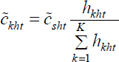
Since we know the hours that each child is in care for each type of care, we split the cost in proportion to the hours spent in that type of care. We assume that families are spending the same amount per hour on each child within the same age range for each type of care. We calculate the net child care cost per child as
(16)
We combine this with the hours of child care information to calculate a gross per-child price for each type of care.
We take all of these individual child prices and calculate two median prices for each Labour Force Survey Region (LFSR): one for children who are not yet in school and one for school-aged children. We impute this median price to each household in the LFSR. For pre-school children, we have sixteen observations per LFSR on average. There is substantial variation across LFSRs. Table 5 in Gong et al. 2010 shows that this method of constructing prices does well in matching state-level average prices from administrative data.
By using local area averages, we are essentially using a quality-adjusted price. Our modelling assumption is that households react to the average price level irrespective of the quality they choose. This is akin to assuming that shifts in median prices affect all quality levels. We control for child care quality by adding variables from administrative data which capture the average number of qualified staff per child in formal day care centres. These variables are only available at the state level however.
Finally, we note that the main variable of interest in this study is the price of child care for children who are not yet in school. We calculate the price for school-aged children and this price enters into the family budget constraint (and thus it affects the decision to work), but we do not analyse how changes in this price affect behaviour. We focus on how mothers' behaviour changes as the price for pre-school children changes.
7 See Watson and Wooden (2002) for more details.
8 For an explanation of the difference between the gross and net child care price indexes, see 'Child Care Time Series Table' in 'Appendix Child Care Services in the CPI. Treatment of Child Care Services in the Australian Consumer Price Index (CPI)' in Australian Bureau of Statistics, 2010 (Last viewed 20 July 2011.)
9 We use the median since it is less vulnerable to outliers than the mean.
10 Labour Force Survey Regions are described in ABS, 2005.
11 This last category is mostly in-home care at the home of the carer or the home of the child.