David Gruen, Bonnie Li and Tim Wong1
The resources boom, globalisation and other global economic forces have raised questions about whether employment and unemployment outcomes in regional Australia have become more unequal. This paper examines how the dispersion of unemployment across regions has changed over time. Our results show that unemployment dispersion has narrowed as the aggregate level of unemployment has declined. This relationship has not changed over the course of the current resources boom and is consistent with similar outcomes in the United States and the United Kingdom.
Introduction
Over the past decade, Australia’s increasing integration with emerging Asian economies has led to a sustained surge in demand for our resource commodity exports on a scale never seen before. This has led to rapid growth in the mining and mining-related sectors and relevant regions while placing pressure on other parts of the Australian economy (Gruen 2011). Added to this, there have been increasing concerns around the employment outlook in some industries competing with Asian producers, whose emergence as major players in the global trading system has accelerated.
This paper seeks to inform this debate by examining whether strong aggregate employment outcomes have masked increasingly disparate outcomes between Australian regions. In particular, building on the work of Thirlwall (1966), we examine how unemployment has been distributed and how its dispersion has changed since the 1990s.
Our results show that unemployment disparity across Australian regions has fallen as the aggregate rate of unemployment has declined. This strong relationship has not changed over the course of the current resources boom. We find a similar strong, positive relationship between the dispersion of regional unemployment rates and the aggregate unemployment rate in both the United Kingdom (UK) and the United States (US).
The paper is structured as follows: first we present a brief review of unemployment outcomes in Australia, with a particular focus on differences between mining and non-mining states. We then explore unemployment distribution and dispersion at the regional level for Australia. This analysis is then extended to examine unemployment distribution in the UK and the US.
Setting the scene — trends in unemployment
Since the onset of the resources boom in the early 2000s, Australia’s terms of trade — that is, the ratio of export to import prices — has surged to historically high levels. The combination of surging export prices for Australian commodities and the constrained growth in import prices faced by Australians has boosted real national income and purchasing power (Parkinson 2011).
The strong boom has prompted discussion of a two-speed economy. In particular, the resources boom is benefiting mining and mining-related sectors as well as the states and territories where these are concentrated, while restraint has been placed on other parts of the economy.
While a two-speed economy is evident in looking at output growth by sector, this need not translate to a widening in employment outcomes between regions. The rise in the terms of trade affects the economy in two main ways: through a resource movement effect and a spending effect (see, for example, Corden 1984, Corden and Neary 1982 and Gregory 1976). In particular, as the mining sector demands more labour and capital, it utilises any spare capacity in the economy and draws resources away from lagging sectors. In addition, the extra income and government revenues from the higher terms of trade increases demand for goods and services. This in turn raises demand for labour in the sectors not exposed to international competition. It remains an empirical question whether the combined effect of these two forces has a favourable or adverse effect on unemployment disparity across regions.
Not surprisingly, the resources boom has provided a greater stimulus to activity in the mining states than elsewhere (Garton 2008).2 Since 2003-04, gross state production (GSP) has on average grown around 1.7 times as fast in the mining states as in the non-mining states. Over the same period, for each 1 per cent increase in employment in the non-mining states, employment has also increased by around 1.7 per cent in the mining states (Chart 1).
Chart 1: Employment growth in Australia
Year average
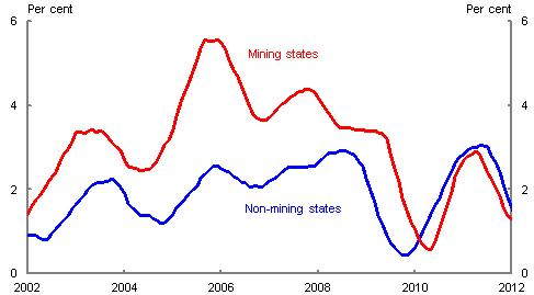
Source: Australian Bureau of Statistics (ABS, cat. no. 6202.0) and Treasury.
The stronger growth in the mining states has also led to a more rapid decline in the unemployment rate in those states. As highlighted by Garton (2008), this has reversed previous experiences — where mining states had higher unemployment rates. The unemployment rate in the mining states was 1 percentage point lower than in the non-mining states’ prior to the onset of the global financial crisis (Chart 2).
Although the unemployment rate in the mining states fell below that in the non-mining states in the mid 2000s, unemployment across both groups has fallen since the late 1990s and has stabilised at similar levels following the global financial crisis.
Chart 2: Unemployment rate in Australia
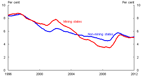
Source: ABS cat. no. 6202.0 and Treasury.
Unemployment disparity across regions
The distribution of regional unemployment in Australia
While unemployment disparity has fallen at the state level, it is also of interest to examine unemployment disparity at a more disaggregated level.
For Australia, we can examine unemployment outcomes across Statistical Local Areas (SLAs) using quarterly Small Area Labour Market data from the Department of Education, Employment and Workplace Relations (DEEWR) for the period 1990 to 2011.3
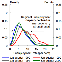
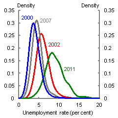
We find that unemployment disparity across Australian (SLA) regions has narrowed as aggregate outcomes have improved over the 1990s (Chart 3). As Australia emerged from the early 1990s recession, the variation in regional unemployment rates narrowed as the national rate declined. In the June quarter 1992, around 10 per cent of Australia’s (SLA) regions recorded an unemployment rate of 5 per cent, and only around 15 per cent of the regions had unemployment rates within a band of 1 percentage point either side of the national average. By the June quarter 1996, the proportion of regions with unemployment rates below 5 per cent had risen to around 21 per cent, while the proportion of regions with unemployment rates within the 1 percentage point band had risen to 20 per cent. By the June quarter 2000, the corresponding figures were 34 per cent and 21 per cent respectively.
Chart 3: Unemployment distribution in Australia
Before the resources boom
During the resources boom
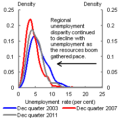
Note: Regional distributions are smoothed using Gaussian kernel density estimation (see, for example, Wand and Jones 1995). For prese
ntational clarity, distributions were deliberately over‑smoothed with windows of 1 for the selected quarters before the resources boom, and windows of ¾, ½ and ¾ for the December quarters 2003, 2007 and 2011 respectively.
Source: DEEWR and Treasury.
Since the beginning of the resources boom in the early 2000s, these trends have remained intact. Demand for labour has increased in the mining and related sectors (for example, the construction and business services sector). These sectors have drawn labour from other parts of the economy which are not directly exposed to the resources boom. Across both mining and non-mining communities, unemployment has declined.
Overall, the distribution has narrowed and shifted to the left since the early 2000s. However, as the effects of the global financial crisis hit the labour market, the distribution widened and became less even. The subsequent general economic recovery and re-emergence of the resources boom have resulted in a further narrowing of the density more recently.
As of the December quarter 2011, the national unemployment rate was 5.1 per cent and around 57 per cent of the (SLA) areas had an unemployment rate of 5 per cent or less. While current labour market conditions are not as strong as those that prevailed just before the global financial crisis, they are considerably stronger than those before the resources boom, with lower average unemployment and a more even distribution. For instance, as of the December quarter 2002, there were only around 24 per cent of the areas with unemployment rates within 1 percentage point of the national average. This is considerably lower than the proportion as of the December quarter 2011 of just below 30 per cent and around 32 per cent prior to the global financial crisis. Hence, the distribution of unemployment distribution across regions has become more even.
Measuring dispersion in these distributions
One of the ways of quantifying the ‘evenness’ of the distribution of unemployment is to measure its dispersion.
There are different approaches to measuring dispersion. The most commonly used measures are the standard deviation and the coefficient of variation of the regional unemployment rates weighted by the corresponding labour force sizes. They are referred to as the absolute dispersion and relative dispersion of unemployment rates.
The absolute dispersion measures the variation of regional unemployment rates around the national unemployment rate, whereas the relative dispersion measures the variation of regional unemployment rates relative to the national unemployment rate (see Appendix A for the computation of the two measures).
The two dispersion measures may diverge and do not necessarily yield similar trends (see Box 1). The absolute measure is more resistant to movements in the aggregate unemployment rate, which makes it more comparable over time (see, for example, Thirlwall 1966). For the purpose of examining dispersion in unemployment outcomes, this paper uses the absolute measure. 4
Box 1: The difference between absolute and relative dispersion measures
Suppose there are three regions (A, B, and C) of equal labour force size in the economy, and that the unemployment rates in these regions are 2, 3 and 8 per cent respectively (Table 1).
If all the regions see an increase in unemployment rates of 1 percentage point (Scenario 1), then the absolute dispersion would remain unchanged, but the relative dispersion would fall. However, if the unemployment rate were to double for all regions (Scenario 2), the absolute dispersion would also double, while the relative dispersion would stay constant and, as a result, would not capture the amplified gaps between regions.
Most distinctly, if the unemployment rate in Region B rises from 3 per cent to 8 per cent, making unemployment outcomes more polarised, the relative measure is lower compared to the original situation rather than being higher (Scenario 3).
| Original | Scenario 1 | Scenario 2 | Scenario 3 | ||
|---|---|---|---|---|---|
| Unemployment rate (per cent) | Region A | 2 | 3 | 4 | 2 |
| Region B | 3 | 4 | 6 | 8 | |
| Region C | 8 | 9 | 16 | 8 | |
| Aggregate unemployment rate (per cent) | 4.3 | 5.3 | 8.7 | 6 | |
| Absolute dispersion (percentage points | 3.2 | 3.2 | 6.4 | 3.5 | |
| Relative dispersion (per cent) | 74.2 | 60.3 | 74.2 | 57.7 |
Note: Appendix A outlines the computation of dispersion.
Thus, the absolute and relative dispersion measures do not necessarily move in line with each other. The divergence is due to the scale insensitivity and location sensitivity of the coefficient of variation. Owing to these characteristics, to avoid unnecessary complication and potential misinterpretation, researchers caution against using relative dispersion (see, for example, Livers 1942, Bedeian and Mossholder 2000, and Sørensen 2002).
In spite of this, there has been some confusion in the literature around these two measures. Some studies have interpreted a negative relationship between the relative unemployment dispersion and the unemployment rate as a negative relationship between the absolute unemployment rate dispersion and the aggregate unemployment rate. As such, they have been led to incorrectly claim that lower unemployment has been achieved at the cost of increased (absolute) dispersion in unemployment rates across regions.
Regional unemployment dispersion and aggregate unemployment
An increase in demand for labour in a region will see unemployment in that region fall, which will encourage higher workforce participation. If this demand cannot be met, employers will adjust wages to attract new workers including those from other regions. This effectively reduces available labour and leads to a fall in unemployment in these other regions. Hence, we would expect a lower degree of dispersion; albeit with a lag (see, for example, Debelle and Vickery 1998). As such, we would expect a positive relationship between aggregate unemployment and unemployment dispersion.
Unemployment dispersion in Australia has narrowed over the past decade (Chart 4). While the dispersion picked up moderately during the global financial crisis, it remained low and has declined since. This suggests that the gains from the resources boom, in terms of unemployment outcomes, have been broadly distributed throughout the country.
Chart 4: Labour market trends in Australia
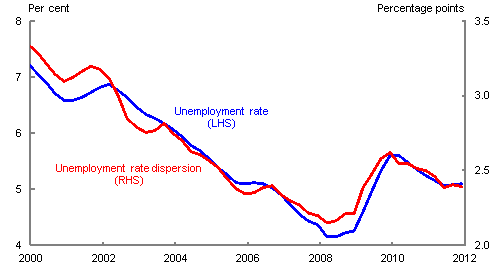
Source: DEEWR and Treasury.
We noted above that there are reasons to expect the dispersion of regional unemployment rates to be positively related to the national unemployment rate. Indeed, when we compare the unemployment rate dispersion with the unemployment rate, they move very closely over time (Chart 4). This is also consistent with earlier studies in Australia (see, for example, Andrews and Karmel 1993).
To examine the relationship between unemployment dispersion and unemployment more clearly, we plot the unemp
loyment rate dispersion against the national (aggregate) unemployment rate (Chart 5). As expected, there is a clear positive relationship, with lower unemployment rates associated with lower levels of dispersion in unemployment rates. 5
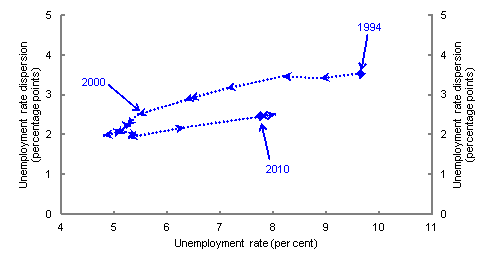
Chart 5: Unemployment rate dispersion and unemployment rate in Australia
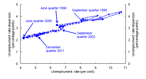
Note: Each small arrow points to the following observation. There are several missing observations between the June quarter 1990 and the June quarter 1998. The diamonds represent the June quarter 1990 and the December quarter 2011.
Source: DEEWR and Treasury.
International comparison: the UK and the US
In the previous section, we presented our findings that highlighted the tendency for the unemployment rate dispersion to move in the same direction as the unemployment rate in Australia. This section investigates whether this relationship also exists in the UK and the US.
For the UK, we examine the distribution of unemployment across around 200 counties and equivalents with Annual Population Survey data from the Office for National Statistics (ONS) since 1995. For the US, we use data from the Bureau of Labor Statistics (BLS) for around 3,200 counties and equivalents since 1990, in addition to state data from the mid-1970s.
The distribution of regional unemployment in the UK and the US
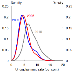
In both the UK and the US, unemployment and unemployment dispersion were at similar levels in 2007 as they were in the early 2000s (Chart 6). The US had seen some improvement in employment outcomes in 2007 relative to 2002, mainly due to the recovery from the bursting of the dot-com bubble.
Since the crisis, the distribution of unemployment has been more uneven for both the UK and the US (Chart 6). In particular, around half of the US counties had an unemployment rate within 1 percentage point of the national average in 2007. This compares to only around a quarter of the counties in 2011. Similarly for the UK, around 40 per cent of the counties had an unemployment rate within the 1 percentage point range in 2007. This proportion has fallen markedly since the global financial crisis to only around 25 per cent in 2010.
Chart 6: Unemployment distribution in the UK and the US
UK
US
Note: County or equivalent data used for both the UK and the US. The UK chart represents averages over the years beginning in March 2002, April 2007 and April 2010, whereas the US chart represents averages over calendar years. Similar to Chart 3, regional distributions are smoothed using Gaussian kernel estimation (see, for example, Wand and Jones, 1995). For presentational clarity, distributions were delibrately over-smoothed with windows of 1 for the UK and ¾ for the US.
Source: ONS, BLS and Treasury.
Unemployment dispersion
As for Australia, a positive relationship between the unemployment rate and the dispersion of regional unemployment rates is also found in the UK and the US (Charts 7 and 8). This is consistent with the findings of many other researchers (see, for example, Martin 1997, and Valletta and Kuang 2010).
However, there appears to be one exception — the dot-com bubble in the early 2000s. While the US unemployment rate increased by around two percentage points after the bursting of the bubble, unemployment rate dispersion increased only marginally. Unemployment dispersion has otherwise been considerably more sensitive to economic slowdowns.
Chart 7: Unemployment rate dispersion and unemployment rate in the UK
Note: Each small arrow points to the following year which begins in March for 1995 to 2003 and April for 2004 to 2010. The diamonds represents the years beginning March 1994 and April 2010.
Source: ONS and Treasury.
Chart 8: Unemployment rate dispersion and unemployment rate in the US
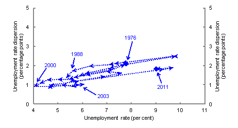
Note: Each small arrow points to the following calendar year. The diamonds represent calendar years 1976 and 2010. State data used for the chart.
Source: BLS and Treasury.
There have been a number of periods during which the relationship between the dispersion of regional unemployment rates and the unemployment rate in the UK and the US appears to have changed. For example, the UK saw a fall in the unemployment rate dispersion relative to the unemployment rate in the early 2000s. This followed the New Deal welfare reform launched in 1998 which changed the labour market landscape (see, for example, Beaudry 2002, and Riley and Young 2001). For the US, there were two shifts in the late 1980s and the late 1990s to lower dispersion, but an unfavourable shift towards higher dispersion in the early 1990s. These changes reflect the influence of factors other than changes in the unemployment rate, such as impacts of public policy and technological change.
Conclusion
Unemployment disparity tends to move in line with unemployment in Australia, the UK and the US.
For Australia, this relationship has held up over the past 20 years amid significant structural changes in the economy and the variation in the growth rates across industries. During the resources boom, the deviation in regional unemployment rates has narrowed as the national unemployment rate has fallen.
Appendix A: The computation of absolute and relative unemployment rate dispersion measures
The absolute dispersion of unemployment rates (AD) is often measured by the standard deviation of the regional unemployment rates from the national average weighted by the corresponding region’s labour force size, that is:
![]()
where ![]() and
and ![]() are the unemployment rate and labour force size of the
are the unemployment rate and labour force size of the ![]() -th region,
-th region, ![]() denotes the aggregate unemployment rate and
denotes the aggregate unemployment rate and ![]() is the aggregate labour force.6
is the aggregate labour force.6
The relative dispersion of unemployment rates (RD) is measured by the coefficient of variation in the regional unemployment rates with respect to the national unemployment rate. It can be calculated as:
![]()
![]()
This paper uses the absolute dispersion to measure unemployment dispersion across regions.
Appendix B: Focusing on regions with unemployment rates above national average
In theory, the truncation of the distribution of unemployment rates at zero could be responsible for our observed correlation between the aggregate unemployment rate and its dispersion.
To see whether this is a genuine issue, we restrict the sample to those regions with unemployment greater than the national average and measure the spread from the national average — that is:
![]()
where the symbols have the same definition as in Appendix A.
For these regions, we find again a positive relationship between dispersion of unemployment rates from the national average and the national unemployment rate (Chart 9). We find similar results for the UK and the US.
This result provides strong evidence that unemployment outcomes are distributed more evenly across regions when the national unemployment rate is lower, and that this outcome is not a statistical artefact.
Chart 9: Unemployment rate dispersion and unemployment rate in Australia
Selected regions
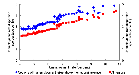
Note: There are several missing observations between the June quarter 1990 and the June quarter 1998.
Source: DEEWR and Treasury.
References
Andrews, L and Karmel, T 1993, ‘Dynamic aspects of unemployment’, Regional labour market disadvantage, pp 45-105, Australian Government Publishing Service.
Beaudry, R 2002, ‘Workfare and welfare: Britain’s New Deal’, Working paper series 2, York University, UK.
Bedeian, A G and Mossholder, K W 2000, ‘On the use of the coefficient of variation as a measure of diversity’, Organizational Research Methods, 3 (3), pp 285-97.
Corden, W M 1984, ‘Booming sector and Dutch disease economics: survey and consolifation’, Oxford Economic Papers, 36, pp 359-80.
Corden, W M and Neary, J P 1982, ‘Booming sector and de‑industrialisation in a small open economy’, The Economic Journal, 92, pp 825‑48.
Debelle, G and Vickery, J 1998, ‘Labour market adjustment: evidence on interstate labour mobility’, Research Discussion Paper, Reserve Bank of Australia.
Garton, P 2008, ‘The resources boom and the two-speed economy’, Economic Roundup, Issue 3, 2008, pp 17-29.
Gregory, R G 1976, ‘Some implications of the growth of the mineral sector’, The Australian Journal of Agricultural Economy, 61, pp 201-19.
Gruen, D 2011, ‘The macroeconomic and structural implications of a once-in-a-lifetime boom in the terms of trade’, address to the Australian Business Economists, 24 November 2011.
Livers, J J 1942, ‘Some limitations to use of coefficient of variation, Journal of Farm Economics, 24 (4), pp 892-5.
Martin, R 1997, ‘Regional unemployment disparities and their dynamics’, Regional Studies, 31 (3), pp 237-52.
Parkinson, M 2011, ‘The implications of global economic transformation for Australia’, address to the Australian Industry Group National Forum on 19 September 2011.
Riley, R and Young, G 2001, ‘The macroeconomic impact of the New Deal for Young People’, research discussion paper, National Institute for Social and Economic Research.
Sørensen, J B 2002, ‘The use and misuse of the coefficient of variation in organizational demography research’, Sociological Methods Research, 30(4), pp 475-91.
Thirlwall, A P 1966, ‘Regional unemployment as a cyclical phenomenon’, Scottish Journal of Political Economy, 13, pp 205-19.
Valletta, R, and Kuang, K 2010, ‘Is structural unemployment on the rise’, FRBSF Economic Letter, 2010-34 (November 8).
Wand, M P and Jones, M C 1995, Kernel Smoothing, Chapman and Hall, London.
1 We are indebted to: Shane Johnson for his leadership in this project; James Kelly and Ben Dolman for comments and suggestions; and Will Devlin, Stephanie Gorecki and Yong Jortzik-Yan for their assistance. The views in this article are ours and not necessarily those of the Australian Treasury.
2 ‘ is a shorthand for states and territories. ‘Mining states’ include Western Australia, Queensland, and Northern Territory. The remaining states (New South Wales, Victoria, South Australia, Tasmania and the Australian Capital Territory) are then ‘non-mining states’.
3 The number of SLAs has varied over time from around 1,300 in the 1990s to over 1,400 in 2006.
4 For the remainder of the paper, unless otherwise stated, ‘dispersion’ refers to absolute dispersion.
5 While the zero-lower bound in unemployment rates could lead to this result, we find that this is not the case (see Appendix B).
6 The absolute dispersion can also be measured by the average deviation of regional unemployment rates from the aggregate unemployment rate weighted by the corresponding labour force size, which has the form:
![]()
The difference between the average deviation and the standard is in their treatment of the outliers. The quadratic function in the standard deviation focuses more on larger deviations and less on smaller deviations. We find very similar results using this measure.