Forecasting the macroeconomy



Robert Ewing, David Gruen and John Hawkins¹

This article examines Treasury’s macroeconomic forecasting performance over the period from 1989-90 to 2003-04, with a focus on forecasts of nominal and real GDP, the GDP deflator, the unemployment rate, and CPI inflation.

The forecasts show little evidence of bias although, in common with most forecasts, they tend to underestimate large changes. As an important example of this general pattern, the recession of the early 1990s was not forecast. Over more recent years, forecasting errors have been significantly smaller, although this is explained, at least to some extent, by the more stable economic environment since the early 1990s recession.

Over recent years, forecast errors in real GDP and the GDP deflator have tended to offset each other. As a consequence, nominal GDP forecasts have been more accurate than those of either real GDP or the GDP deflator. This has likely occurred because of a predominance of unanticipated supply side shocks over recent years, which have moved real output and prices in opposite directions. The forecasts of CPI inflation have been significantly more accurate than those of the GDP deflator, suggesting that the broader basket of economy-wide prices that together make up the GDP deflator are particularly difficult to forecast.

Introduction

Treasury forecasts the macroeconomy as part of the process of forecasting expenditure and revenue for the budget, and more broadly to assist in the framing of forward-looking policy advice.² Far from being a perfect science, macroeconomic forecasting is in some ways more of an art. Predicting human behaviour is inherently more difficult than predicting physical phenomena. The speed of light is constant and can be measured precisely; not so the marginal propensity to consume. It is challenging to capture the key features of a complex modern economy in a framework simple enough to be tractable. Economies are subject to gradual structural change and buffeted by a range of shocks. Collection lags and revisions mean that forecasters can do no better than make informed estimates of the current state of the economy; by contrast for example, weather forecasters can at least be sure about whether or not it is currently raining. In short, ‘economic forecasters aren’t stupid; what we are trying to do is hard’; Gruen (2000).

Part of the process of improving forecasting performance involves assessing past performance. This article reviews Treasury’s forecasting performance for some of the major economic aggregates over the period since 1989, with a particular focus on nominal GDP and its components, real GDP and the GDP deflator. This focus is part of a substantial effort within Treasury to improve the quality of the forecasts of nominal GDP, which are an important input into forecasts of taxation revenue.

Treasury conducts four forecasting rounds each year. In each round, forecasts are generated for (at least) the current and next financial years. As a consequence, the outcome for each macroeconomic aggregate in each year is forecast many times. The two major forecasting rounds form the basis for the forecasts published in the budget papers and in the Mid-Year Economic and Fiscal Outlook (MYEFO). The quality of forecasts can be measured in a number of ways, but most approaches tend to yield similar results. Box1 discusses the two measures used throughout this paper, which measure the bias and accuracy of a set of forecasts.

Gross domestic product

Gross domestic product (GDP) is a key macroeconomic variable. Treasury forecasts both nominal (current price) and real (chain volume) GDP. Nominal GDP measures the value, in current dollars, of the economy’s aggregate production of goods and services, while real GDP is a measure of the quantity of goods and services produced, and hence is a measure of the aggregate level of activity in the economy.

Nominal GDP

Table 1 shows how Treasury’s forecasts of year-average nominal GDP growth have performed relative to the Australian Bureau of Statistics’ (ABS) first published estimates of the outcomes. Table 2 shows the performance of the same set of forecasts, but this time compared to the ABS’s most recent estimates of the outcomes.³

Table 1: Performance of nominal GDP growth forecasts against first published outcomes

1. Only the final four of the six forecasting rounds are available for 1989-90.
2. Mean absolute percentage error, see Box 1 for description.
3. March forecast round for the financial year starting in July of the same year.
4. September forecast round for the financial year that started two months earlier.

Table 2: Performance of nominal GDP growth forecasts against most recent estimated outcomes

1. Only the final four of the six forecasting rounds are available for 1989-90.
2. Mean absolute percentage error, see Box 1 for description.
3. March forecast round for the financial year starting in July of the same year.
4. September forecast round for the financial year that started two months earlier.

The mean error in the forecasts depends importantly on whether they are compared with the first-published or most recent estimated outcomes. On average over the full sample, Treasury’s nominal GDP growth forecasts are 0.54percentage points higher than the first-published outcomes but only 0.15percentage points higher than the most recent estimated outcomes. On average over the more recent period, 1995-96 to 2003-04, the forecasts are 0.10 percentage points lower than the first-published outcomes, but 0.44percentage points lower than the most recent estimated outcomes.⁴

Box 1: Measures of forecasting performance Two commonly used measures of forecasting performance are the mean error and the mean absolute percentage error. For growth rates these are calculated as:
where is the actual growth rate for the variable in period i, is the forecast for growth in that period, both in percentage points, and n is the number of observations. The means can then be calculated for several years, and over several different forecast rounds. The mean error measures the bias of the forecasts. A positi ve number indicates that, on average, the forecast tended to be larger than the outcome (overestimation bias) while a negative number indicates forecasts tended to be smaller than the outcome (underestimation bias). The mean absolute percentage error measures the accuracy of the forecasts, as it measures the average distance between the forecast and the outcome. For both bias and accuracy, a smaller number indicates a better forecasting performance. The main alternative is root-mean-square-error, which accords more importance to large misses. Most studies, such as Zarnowitz (1991) for the United States and Holden and Peel (1988) for the United Kingdom, find that conclusions are insensitive to the choice of measure. For cases where both measures may be misleading, see Macfarlane and Hawkins (1983). Measures of bias and accuracy should be interpreted in the light of the series being forecast. Clearly, the average magnitude of the growth rate is important — a onepercentage point bias in a series that grows on average by 40percent is a very different performance to a onepercentage point bias in a series that grows on average by 2percent.

These differences occur because the ABS has revised up year-average nominal GDP growth outcomes from the first-published to the most recent (December quarter 2004) estimates by an average of 0.3 percentage points over the period. Virtually all of this is an upward revision to estimates of real GDP growth, rather than the GDP deflator.

For the remainder of this article we focus attention on comparing the forecasts with the most recent estimated outcomes as they presumably represent the ABS’s current best estimates of the true outcomes. This is in line with the view that ‘the main object of forecasting is to anticipate what will actually happen in the economy rather than what the data source agencies, on the basis of incomplete information, initially estimated had happened’; McNees (1981).⁵

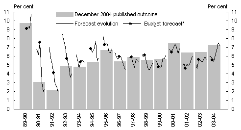
Chart 1 shows the evolution of Treasury’s forecasts for year-average nominal GDP growth over the past fifteen years, as well as the most recent estimates of the outcomes. For some years, the last forecast differs noticeably from the outcome as we understand it today. This is usually because of significant revisions to the estimated outcome between the first and most recent National Accounts releases.⁶

The columns in the chart show the year-average GDP growth currently estimated by the ABS, and the lines show the evolution of the forecasts for that financial year over successive forecasting rounds. The first point on the line for each financial year shows the first forecast, usually made around two years before the end of the financial year in question (for instance, the first point on the line for 2003-04 is the forecast made in September 2002). The dot on each line shows the budget forecast for that financial year. It does not always appear at the same point on the line, as the budget moved from August to May in 1994, where it has remained, with the exception of the 1996 budget which was brought down in August.

As Chart 1 makes clear, most of the forecasting error, and the bias, arise from the first few years of the period, particularly 1990-91, 91-92 and 92-93. The recession of 1990-92 was not forecast and, as a result, nor was the speed of the transition to the new low-inflation environment.⁷

The visual impression left by Chart 1 is confirmed in the earlier tables which reveal significantly smaller mean absolute percentage errors (MAPEs) over the more recent years, 1995-96 to 2003-04, than over the earlier years.

Chart 1: Evolution of nominal GDP growth forecasts

* For example, the 1993-94 budget forecast for 1993-94.

Source: Australian Bureau of Statistics 2004, National Income Expenditure and Product, cat. no. 5206.0, December, Canberra. Treasury forecasts.

Real GDP

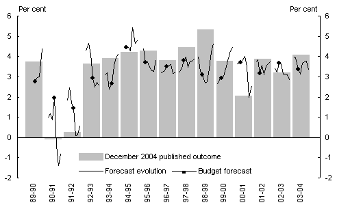
Summaries of Treasury’s overall forecasting performance for real GDP growth against the most recent estimated outcomes are shown in Table 3 and Chart 2.

Table 3: Performance of real GDP growth forecasts against most recent estimated outcomes

1. Only the final four of the six forecasting rounds are available for 1989-90.
2. Mean absolute percentage error, see Box 1 for description.
3. March forecast round for the financial year starting in July of the same year.
4. September forecast round for the financial year that started two months earlier.

The forecasts of real GDP show a different picture to the nominal forecasts. Through the 1990-92 recession the forecasts significantly overestimated output initially. The recovery from the recession was forecast fairly accurately, and the size of the forecast errors, as well as the forecast movements in the remainder of the period, has been relatively small.

There are three obvious exceptions to this, namely the forecasts for the years 1998-99, 1999-2000 and 2000-01, where there were relatively large movements in successive forecasts of real GDP. These movements reflect the impact of the Asian financial crisis, and the economy’s response to the introduction of the GST. The Asian financial crisis was initially expected to have more of a contractionary effect on the Australian economy than turned out to be the case. By contrast, following the introduction of the GST, there was a bigger fall in activity in the dwelling sector than was expected.

Chart 2: Evolution of real GDP growth forecasts

Source: Australian Bureau of Statistics 2004, National Income Expenditure and Product, cat. no. 5206.0, December, Canberra. Treasury forecasts.

GDP deflator

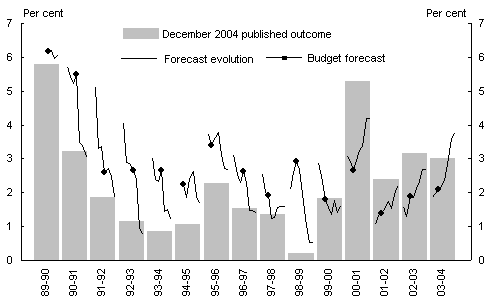
The GDP deflator is a measure of the aggregate prices of goods and services produced in Australia. Its growth rate is (approximately) the difference between growth in nominal and real GDP. Summaries of Treasury’s overall forecasting performance for growth in the GDP deflator against the most recent estimated outcomes are shown in Table 4 and Chart 3.

Table 4: Performance of GDP deflator growth forecasts against most recent estimated outcomes

1. Only the final four of the six forecasting rounds are available for 1989-90.
2. Mean absolute percentage error, see Box 1 for description.
3. March forecast round for the financial year starting in July of the same year.
4. September forecast round for the financial year that started two months earlier.

Chart 3: Evolution of forecasts of growth in the GDP deflator

Source: Australian Bureau of Statistics 2004, National Income Expenditure and Product, cat. no. 5206.0, December, Canberra. Treasury forecasts.

Table 4 shows a very small mean error over the period from 1995-96 to 2003-04, but this is somewhat misleading as it arises from a rough cancelling of the overestimation in the late 1990s by the underestimation in the early 2000s. The MAPE is similar in these two sub-periods.

Growth in the GDP deflator was initially overestimated in every year from 1989-90 to 1999-2000, although the size of the overestimate fell on average through the decade. And then from 2000-01 to 2003-04, growth in the GDP deflator was significantly underestimated in every year (Chart 3). In several years, the last forecast differs substantially from the most recent estimate of the outcome; this arises largely because of revisions from the first-published to the most recent estimate of the outcome.

Towards an understanding of the forecast errors

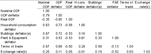
Table 5 shows correlation coefficients between March forecast errors for nominal GDP growth and some of its main determinants over the years 1995-96 to 2003-04.⁸ For each variable, the forecast error is the difference between its March forecast and its latest estimated outcome (though a different definition is appropriate for the exchange rate— see note (b)).

Table 5: Correlation coefficients between March forecast errors, 1995-96 to 2003-04

1. Deflator for residential and non-residential buildings and ownership transfer costs.
2. The exchange rate assumption is the average value of the TWI in the month before the March round forecasts are finalised. The outcome is not revised.

There is a strong negative correlation (-0.85) between the forecast errors for GDP deflator growth and real GDP growth. A strong negative correlation is also observed between the forecast errors for the same variables using forecasts produced by Access Economics at roughly the same times as the Treasury forecasts. These negative correlations suggest a predominance of unanticipated supply shocks over the period, since these shocks tend to move output and prices in opposite directions. Further analysis of this strong negative correlation seems a worthwhile exercise for the future.

A consequence of the strong negative correlation is that the nominal GDP growth forecasts have a smaller MAPE than the forecasts of either GDP deflator growth or real GDP growth. The MAPE for the March forecasts over the period, 1995-96 to 2003-04, is 1.22 for GDP deflator growth, 0.92 for real GDP growth but only 0.85 for nominal GDP growth (see earlier tables).

The March forecast errors for nominal GDP growth are strongly positively correlated with the forecast errors for household consumption deflator growth, buildings deflator growth, and terms of trade growth (Table 5). Forecast errors in household consumption deflator growth and buildings deflator growth feed straightforwardly into errors in GDP deflator growth, and hence into errors in nominal GDP growth. However, the mechanism by which forecasting errors in terms of trade growth typically translate into forecasting errors in GDP deflator growth, and hence into errors in nominal GDP growth, is more complicated, and worth explaining.

Consider a typical forecasting error in terms of trade growth. For concreteness, assume that the March forecast is for the year-average terms of trade to remain flat over the coming financial year, but the outcome turns out to be a significant rise, driven by a strong unanticipated rise in world commodity prices. If there was no response by the Australian dollar exchange rate to the rise in world commodity prices, then the Australian dollar price of exports would have risen, which would feed directly into higher GDP deflator growth than had been forecast. This story is simple enough.

Typically, however, the exchange rate appreciates significantly with the rise in world commodity prices. As a consequence, there is a smaller (if any) rise in the Australian dollar price of exports than the rise in world commodity prices in foreign currency terms. At the same time, the Australian dollar price of imports falls as the exchange rate rises.⁹ If this fall in import prices was immediately passed through into the domestic prices faced by final users (consumers and firms, in particular) then there would be no first-round effects on the price of domestic production, the GDP deflator (although there would still be positive income effects on the economy from the rise in the terms of trade).

In reality, however, the pass-through of import price changes to final prices is very gradual (especially to final consumer prices). While the gradual pass-through of a fall in import prices is under way, intermediaries along the chain from the docks to the shops experience a rise in their profit margins which contributes directly to a rise in the GDP deflator that was not previously forecast, and therefore to a rise in nominal GDP growth.

Other major economic variables

Unemployment rate

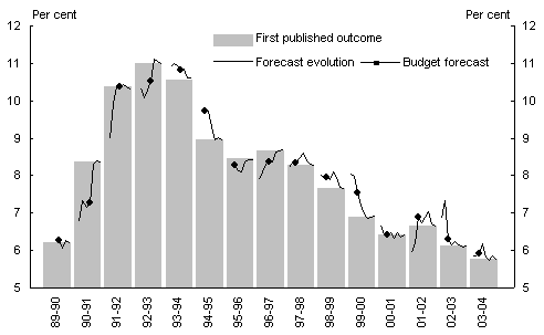
Table 6 and Chart 4 show the performance of Treasury’s forecasts of the year-average unemployment rate for each financial year. Unlike the other variables in this article, the unemployment rate forecasts are compared to the first published outcomes. The majority of revisions to the unemployment rate between the first and most recent publications are due to changes in the definition of unemployment. As each forecast was made on the basis of a particular definition of unemployment, the most appropriate comparison is with the unemployment rate estimated at that time.

The forecasts for the unemployment rate show little overall bias. They do show some degree of conservatism, where the size of movements (both positive and negative) is consistently underestimated.¹⁰ Through the early 1990s recession, the rise in the unemployment rate was consistently underestimated; more recently the fall in the unemployment rate was underestimated through periods when it was falling.

Table 6: Performance of unemployment rate forecasts against first-published outcomes

1. Only the final four of the six forecasting rounds are available for 1989-90.
2. Mean absolute percentage error, see Box 1 for description.
3. March forecast round for the financial year starting in July of the same year.
4. September forecast round for the financial year that started two months earlier.

Chart 4: Evolution of unemployment rate forecasts

Source: Australian Bureau of Statistics 2004, Labour Force, cat. no. 6202.0, Canberra. Treasuryforecasts.

Turning points are difficult to predict, as they require a forecast not only of the rate of growth, but also of the timing of the turning point. The performance of the unemployment rate forecasts is mixed in this regard. While the turning point in 1992-93 was predicted fairly well, the return to declining unemployment in 1998-99 wa
s not, and similarly the start of the recent decline in the unemployment rate in 2002-03 was initially missed.

Consumer Price Index

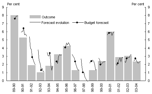
Table 7 and Chart 5 show the performance of forecasts of year-average Consumer Price Index (CPI) inflation. Unlike the other variables discussed in this article, the CPI is not subject to revision. Hence the first estimate published by the ABS is always the same as the most recent estimate.

The first half of the 1990s shows a similar pattern of errors to those for the GDP deflator. The transition to, and sustainability of, low inflation in the early 1990s took time to be recognised in the forecasts. By contrast, from the late 1990s onwards, forecasts of CPI inflation have been very close to the outcomes. This can be attributed, in part at least, to the greater stability of the CPI in this more recent period, which in turn reflects greater experience with the 2to3percent medium-term inflation target.

Table 7: Performance of CPI inflation forecasts against outcomes

1. Only the final four of the six forecasting rounds are available for 1989-90.
2. Mean absolute percentage error, see Box 1 for description.
3. March forecast round for the financial year starting in July of the same year.
4. September forecast round for the financial year that started two months earlier.

Chart 5: Evolution of Consumer Price Index forecasts

Source: Australian Bureau of Statistics 2004, Consumer Price Index, cat. no. 6401.0, December, Canberra. Treasury forecasts.

A comparison of mean absolute percentage errors reveals that Treasury forecasts have been significantly more accurate for CPI inflation than for the broader basket of economy-wide prices that together make up the GDP deflator.

One noteworthy year is 2000-01, when inflation was likely to be difficult to forecast due to the introduction of a new tax system, which had a widespread impact on prices. As events turned out, the CPI forecasts were remarkably close to the outcome — indeed closer than in many other years — although the GDP deflator forecasts were not (Chart3).

The impact of major shocks on forecasting

Unexpected shocks cannot, by definition, be forecast. From a forecasting perspective, the interesting question is how the forecasts adjust to the new information and economic circumstances provided by the shock. Since 1989 there have been many shocks to the Australian (and world) economy. Two of the more recent of these were the Asian financial crisis in 1997-98, and the introduction of the GST in 2000.

The Asian financial crisis broke out in July 1997, soon after the 1997 budget forecasts were released.¹¹ Like other forecasters, Treasury had not foreseen the large devaluations of a number of Asian currencies and the subsequent contractions in their economies. The MYEFO released in December 1997 did not change the forecast for Australian real GDP growth in 1997-98, arguing that weaker external demand would be offset by stronger domestic demand, boosted by interest rate cuts. Somewhat weaker growth of 3 per cent was forecast for 1998-99. Again like other forecasters, Treasury initially underestimated the impact of the Asian crisis on the affected countries, arguing in terms of just a slowing rather than the large contractions in output which eventuated. The forecast for Australian real GDP growth in 1998-99 was lowered marginally in the May 1998 budget, and again in the September Pre-election Economic and Fiscal Outlook to 2percent. The forecast was restored to 3 per cent in the subsequent December MYEFO, which many commentators regarded as optimistic given the impact the crisis was by then having on Australia’s Asian trading partners. In the event, these forecasts significantly underestimated the outcome — the Australian economy was remarkably unaffected by the Asian crisis and real GDP grew by 5per cent in 1998-99.

Major changes to the Australian tax system, most notably a goods and services tax and large cuts in income taxes, were introduced in July 2000.¹² The budget forecasts in May 2000 incorporated some strengthening of consumption and dwelling investment before the tax changes came into effect, at the expense of some forecast weakening after they came into effect. This bringing forward and subsequent unwinding of dwelling investment turned out to be considerably greater than expected. With a rise in interest rates also dampening the sector (as a technical assumption, the budget forecasts are predicated on constant interest rates), dwelling investment contracted by over 20 per cent in 2000-01. Consumption and business investment were also weaker than expected. The December quarter 2000 national accounts showed a 0.6 per cent contraction in real GDP, which came as a surprise to almost all commentators — see Henry (2001), and real GDP grew by 2 per cent for 2000-01 as a whole.

References

Fildes, R. and Stekler, H. 2002, ‘The state of macroeconomic forecasting’, Journal of Macroeconomics, 24, pp. 435-68.

Goldstein, M. and Hawkins, J. 1998, ‘The origin of the Asian financial turmoil’, Reserve Bank of Australia Research Discussion Paper, 9805, May.

Gruen, D. 2000, ‘Forecasting methods: final observations — economic forecasters aren’t stupid; what we are trying to do is hard!’, in Abelson, P. and Joyeux, R. (eds) Economic Forecasting, Allen & Unwin, Sydney.

Henry, K. 2001, ‘On economists, the economy and fiscal policy’, address to Australian Business Economists, 29 May, Sydney. (available at www.Treasury.gov.au).

Holden, K. and Peel, D. 1988, ‘A comparison of some inflation, growth and unemployment forecasts’, Journal of Economic Studies, 15(5), pp. 45-52.

Keynes, J. M. 1936, The General Theory of Employment, Interest and Money, Cambridge University Press (1973 edition).

Macfarlane, I. and Hawkins, J. 1983, ‘Economic forecasts and their assessment’, Economic Record, 59 (167), pp. 321-31.

McNees, S. 1981, ‘The recent record of thirteen forecasters’, New England Economic Review, Federal Reserve Bank of Boston, September/October, pp. 5-21.

Pagan, A. 2003, Report on Modelling and Forecasting at the Bank of England, January.

Theil, H. 1958, Economic Forecasts and Policy, North Holland, Amsterdam.

Zarnowitz, V. 1991, ‘Has macro-forecasting failed?’, NBER working papers, no 3867.

---

¹ The authors are from Macroeconomic Group, Australian Government Treasury. This article has benefited from comments and suggestions provided by Steven Kennedy, David Parker, Martin Parkinson, Meghan Quinn and Nick Stoney. The views expressed are those of the authors and not necessarily those of the Australian Government Treasury.

² See ‘Economic forecasting: history and procedures’ in the Economic Roundup, Autumn2005 for more on the reasons why Treasury forecasts, and the procedures used.

³ The December quarter 2004 National Accounts release (Australian Bureau of Statistics
cat.no. 5206.0) was the most recent available when this article was written.

⁴ It should be noted, of course, that many more revisions have been applied to the most recent estimated outcomes for the earlier years in the sample than for the more recent years.

⁵ Of course, commentary on forecasts in the press mostly concerns the initial estimates. If the purpose of a forecast is to profit in financial markets, the relevant comparison is also with the initial estimates; Fildes and Stekler (2002). It should be noted that the definition of GDP was changed in 1998. However, this change in definition is not the major cause of revisions for most years, so for our purposes the comparison with the most recent estimated outcomes still seems the most appropriate.

⁶ See Pagan(2003) for the implications of these revisions for forecasting the following year.

⁷ The two factors, real output and prices, make roughly equal contributions to the forecasting error for nominal GDP in 1990-91, with the contribution from the GDP deflator rising to around two-thirds in 1992-93.

⁸ Recall that the ‘March forecast’ is the forecast made in the March forecasting round for the financial year starting in July of the same year. For budgets brought down in May, the budget forecasts are used. These forecasts sometimes differ slightly from the forecasts coming out of the March forecasting round, because of the additional information that becomes available before the budget forecasts are finalised in early May.

⁹ The correlation between forecast errors in the terms of trade and in the exchange rate is 0.50 (Table 5). Furthermore, the correlations between changes in the terms of trade and changes in Australian dollar export and import prices support the generalisations in the text. Over the years 1995-96 to 2003-04, the correlation coefficient between the year-average growth rates of the terms of trade and export prices is close to zero (0.08), while that between the terms of trade and import prices is clearly negative (-0.45).

¹⁰ A general tendency towards conservatism had been noted as early as Keynes (1936, p. 148), and confirmed in studies as early as Theil (1958), who concluded ‘the most important systematic error … is the underestimation of change’, and more recent work such as Fildes and Stekler (2002). Macfarlane and Hawkins (1983) note that this tendency becomes more marked with forecasts over longer horizons, which almost invariably contain a ‘return to normality’ for the out-years.

¹¹ A contemporary account of the crisis is given in Goldstein and Hawkins (1998).

¹² The impact of the tax changes is assessed in an article in the Autumn 2003 issue of the Roundup.