Downloads
***Check against delivery***
As always, it is a pleasure to be here at the Australian Business Economists and, particularly, for my second post–Budget address.
Like my first address 12 months ago, today I would like to discuss some of the challenges confronted in framing the Budget released last week, focusing on three issues that have shaped the pre- and post–Budget debate.
- First, the economic forecasts, in particular what's happening behind those forecasts and how that has made forecasting, and revenue forecasting in particular, more difficult.
- Second, Australia's macro-policy frameworks viewed through the prism of how well we have handled the economic shocks that have affected Australia over the past decade.
- Third, given those frameworks, how the individual arms of policy are calibrated as circumstances change, and how this influences our thinking on returning the budget to surplus.
In addressing these three issues, I will also touch on the risks to the outlook.
Forecasts
The economic outlook
Twelve months ago I outlined our expectation that the economy would grow above trend, but in doing so I also emphasized there were a number of risks, particularly from Europe and United States.
One thing being an economic forecaster teaches is the importance of humility.
While we got much of the outlook right, 12 months on we have to acknowledge that 2011–12 will be weaker than anticipated.
The 2011–12 Budget forecast growth of 4 per cent in 2011–12 and 3¾ per cent in 2012–13. That was revised down at MYEFO to 3¼ per cent in both 2011–12 and 2012–13. While we still have two quarters of National Accounts data to go, it looks like growth in 2011–12 will come in closer to 3 per cent and our best judgement is that 2012–13 will still be around 3¼ per cent (Chart 1).
Chart 1: GDP estimates
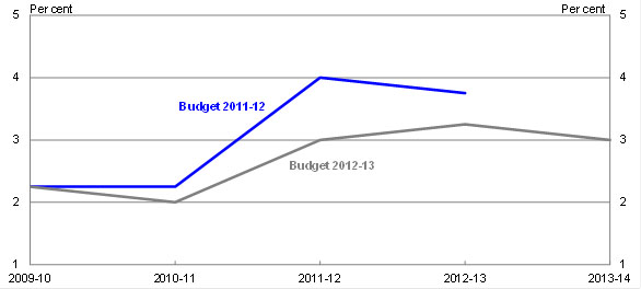
Source: ABS cat. no. 5206.0 and Treasury.
When we look at the 2011–12 Budget forecasts for activity we find that the domestic sector has panned out much as we had expected. Of course there are some compositional differences, as there always are, but it looks like we will be pretty close on the aggregates. At last year's Budget, we forecast total private demand to grow by 6 per cent in 2011–12 and our current expectation is that the outcome will be around 6 per cent.
Table 1: Key Economic forecasts
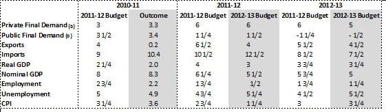
(a) GDP, private final demand, public final demand, exports and imports are year-average growth. Employment and CPI are through-the-year growth to the June quarter.The unemployment rate is the rate for the June quarter.
(b) Excluding second-hand asset sales from the public sector to the private sector.
Our key forecasting error on activity looks to have been around exports and imports.
At last year's Budget, we forecast export growth of 6½ per cent in 2011–12. As it turned out, it looks like it will be closer to 4 per cent. This may not seem much, but exports account for around 20 per cent of GDP so even small errors in the forecasts can have material impacts on the accuracy of the overall GDP forecasts (Chart 2).
Chart 2: Estimates of export and import growth (year-average)
Imports
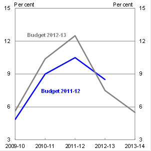
Exports
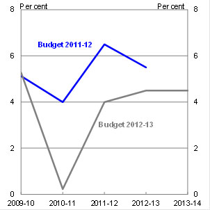
Source: ABS cat. no. 5206.0 and Treasury.
There were a few factors that appear to have contributed to the likely weaker outcomes.
While the global situation has inevitably had an impact, there are also other factors including: our underestimation of how long it would take miners to recover from the 2011 Queensland floods1; an overestimation of how quickly new iron ore and coal capacity could be brought on-line; and the extent of weakness in services exports, particularly education services exports.
While export growth has been weaker than we thought, import growth has been stronger, which translates into a larger net export detraction and lower GDP growth for a given level of final demand growth.
In last year's Budget, we forecast import growth of 10½ per cent in 2011–12. Now it looks like it will be closer to 12½ per cent. The stronger–than–expected import growth predominantly reflects the larger–than–expected business investment growth. As you know resources investment is very import intensive, and the shift towards investment for LNG projects makes it even more so.
Again, this is not much of a miss, given the size of the growth rates. But with imports also equivalent to around 20 per cent of GDP, it still has a material effect on the accuracy of the forecasts.
This highlights one of the complexities of forecasting at the moment. Because of the mining boom, things are moving around much more than usual. Parts of business investment are expected to grow by well over 20 per cent this year; imports are expected to grow by over 12 per cent; and the terms of trade are forecast to fall by more than 10 per cent over the forecast period. Such large movements are difficult to calibrate tightly, but small errors in these components can make a big difference to the accuracy of the forecasts.
We've incorporated the flow of new information — some positive and some negative — into the 2012–13 forecasts. We have also factored in the expected contractionary effect on activity from the Government's fiscal consolidation and the impact of the carbon price.
Not that that necessarily means we will be right. As detailed in Budget Statement 2, there are substantial risks around the forecasts. The global outlook is still very uncertain, as it has been for some time. We are particularly worried by the Euro-zone situation, which is why our forecasts for European growth are markedly weaker than those of the IMF, Consensus and the European Commission (-¾ per cent as against around -¼).
But there are also domestic risks. A key one is around the labour market. The economy is going through a large structural transition and, as noted in Budget Statement 2 (p2-33), there is “the possibility that frictional unemployment could temporarily rise as businesses adjust to changing patterns of demand and workers look to find new opportunities in emerging parts of the economy.”
The labour market is not the only thing that it is difficult to get a handle on at the moment. We know, for example, that the elevated terms of trade and the high exchange rate are having big effects on the broader economy. As are attitudes to debt, changing patterns of consumer spending, competitive pressures and technological change. But, as you would expect, translating the impact of these broad structural forces into precise central case forecasts is particularly challenging.
The revenue forecasts
Forecast errors on the income side also have implications for our tax base.
More subdued outcomes in real and nominal GDP have contributed to nominal tax receipts being weaker than expected, with growth in
nominal GDP revised down for 2011–12 (broadly in line with the downward revision in real GDP) and the 2012–13 forecasts of nominal GDP also revised down.
At last year's Budget, tax receipts were expected to grow by 13.7 per cent in 2011-12. This year's Budget revised that down to 10.3 per cent. This is mainly due to downward revisions to growth in company tax, capital gains tax and consumption taxes.
Company tax receipts were anticipated to rebound very strongly in the 2011-12 Budget by 27.5 per cent. This has been revised down, but to a still robust 19.9 per cent, which reflects several factors.
The first is the implications for company tax of the mining sector growing more rapidly than anticipated and mining investment exceeding expectations.
As set out in Budget Statement 5, these factors will tend to dampen tax receipts as a share of the economy, as mining companies claim tax deductions associated with the depreciation of their capital stock. Of particular importance is the accelerated write-offs provided for many mining assets. Some assets receive immediate deductions while others are depreciated at concessional rates over a longer period. Accelerated write-offs effectively result in the deferral of tax payments into future years. While we had anticipated this factor in our forecasts, we underestimated its magnitude.
Second, it seems that it is taking longer than anticipated for company tax losses to be absorbed. Given the sheer magnitude of losses incurred during the GFC, and the paucity of precedents to guide our judgment about how the losses are utilised, this was always going to be a major forecasting challenge.
Company, superannuation funds' and individuals' income taxes were also affected by capital gains tax (CGT), which was revised down by $1.6 billion between the two budgets.
CGT collections are also affected by the rate at which assets are sold (as it is taxed on realisation not accrual), with considerable volatility from year to year in realisation rates across investors and asset classes.
A further complication stems from the carrying forward of some capital losses into later years which are then used to offset gains. As such, our forecasting methodology requires the tracking of these losses and a calculation of the rate at which they will be utilised. Again, the unprecedented losses from the GFC means there are no well-established historical patterns to draw upon. What this means is that it will take some time to untangle all the reasons for the error in the CGT forecasts.
Indirect tax collections, including GST, have also proven to be weaker than anticipated. These have been revised down $3.7 billion. Conceptually, indirect taxes should track consumption (adjusted for differences in the tax base) fairly closely, but this has not happened in the recent past.
Chart 3: GST and consumption subject to GST
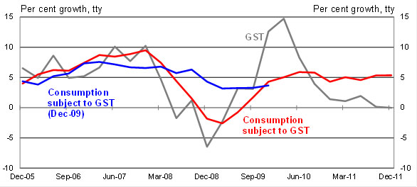
Source: Treasury.
GST collections fell markedly following the onset of the GFC (the grey line in Chart 3). At the time, growth in consumption subject to GST fell only marginally (the blue line) but has since been revised and now better tracks GST growth during 2008 (the red line). There is still, however, a large discrepancy between GST growth and the relevant economic aggregate since 2010. The GST experience suggests that despite a strong bounce-back in 2009-10, consumers remain cautious in their spending.
We expect tax receipts will continue to be affected by changes in the level and composition of the nominal economy, as well as other factors, including asset price growth. Given the significant structural change in the economy, and the changing relationship between the nominal economy and tax collections, this is a particularly challenging time for revenue forecasting.
A robust and flexible macroeconomic framework
I would like to move on to discuss how well our macroeconomic framework — our approach to fiscal policy, monetary policy and the exchange rate — has served Australia in recent times.
Australia has had a medium-term approach to fiscal policy since the mid–1980s, before evolving into a fully articulated framework with the development of the Charter of Budget Honesty in the second half of the 1990s.
A key objective of fiscal policy is to maintain fiscal sustainability from a medium–term perspective. Outside of the automatic stabilisers, discretionary fiscal policy should only be used for supporting demand during extreme circumstances, such as when:
- the effectiveness of monetary policy is impeded; and/or
- a shock is sufficiently large and sufficiently sudden that monetary and fiscal policy should work together effectively to support activity, such as during the GFC.
Monetary policy aims to maintain inflation between 2 and 3 per cent, on average, over the cycle — anchoring inflation expectations. It has the primary responsibility for managing demand to keep the economy on a stable growth path consistent with low inflation.
Put another way, good fiscal and structural policy can create the incentives for supply-side expansion while monetary policy aims to keep demand growing in line with that expansion in potential.
Monetary policy is supported by a floating exchange rate which acts as a shock absorber that offsets some of the effects of global shocks on the economy and naturally adjusts in response to other economic developments.
The medium–term focus of both monetary and fiscal policy, combined with a market–determined exchange rate, is extremely important. It provides great flexibility to deal with the economic shocks that come our way.
Establishing this macroeconomic framework was not easy, and it has evolved through time. But today Australia's macroeconomic policy framework is an asset, an endowment, forming an important part of the economy's productive base.2
Unfortunately it is sometimes forgotten that this framework is in no small part responsible for the relative stability of Australian economic growth for the past two decades. This is despite Australia having faced three of the most significant — some may say the largest — shocks seen since World War II in the past decade.
All three shocks are well known, especially to this audience, but the way that Australia has handled them should not be undersold.
These shocks have tested our macroeconomic framework and resilience and each time we have come through relatively unscathed. In fact, our economic performance in the face of them has been nothing short of remarkable.
Shock 1 — Mining Boom Mark 1
Let me begin with shock 1, otherwise known as Mining Boom Mark 1, which started in the March quarter of 2004. The story of the boom is well known so I won't repeat the details, but I do want to focus on the two arms of macroeconomic policy during this phase, an approach I will repeat in the subsequent two phases.
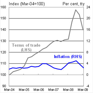
In this shock, rapidly rising demand for Australian mineral resources from China and other emerging economies saw our terms of trade rise by almost 50 per cent from the beginning of 2004 until the eve of the GFC (Chart 4).
Chart 4: Terms of trade
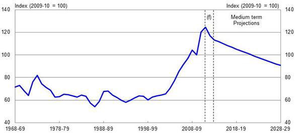
Source: ABS cat. no. 5206.0 and Treasury.
Following a phase of monetary policy easing in the early 2000s in response to the global slowdown following the end of the tech-boom, monetary policy was gradually tightened through the initial phase of the terms of trade boom.
However, with the economy approaching capacity constraints around 2006 and 2007, with
unemployment heading down towards 4 per cent — a rate not seen since the early–1970s, which coincidentally, was the last time Australia experienced a terms of trade boom — the pace of monetary policy tightening increased to address inflationary pressures.
Inflation peaked at 5 per cent in 2008, just before the most dramatic phase of the GFC (Chart 5). At the time the cash rate was 7.25 per cent.
On the fiscal side, the Commonwealth government continued to deliver surpluses in each year between 2002–03 and 2007–08. While the surplus continued to rise each year as a share of GDP, it did so only slightly, suggesting that fiscal policy was recycling a substantial part of the revenue surge back into the economy.3
In addition to the monetary and fiscal policy response, the Australian dollar appreciated from around 76 US cents at the beginning of 2004 to peak at around 95 US cents in June 2008.
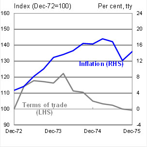
Chart 5: A comparison of Terms of Trade booms
1950s Boom
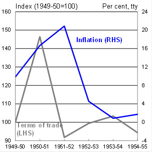
1970s Boom
Source: ABS cat. no 5206.0, 6401.0, RBA and Treasury.
Mining Boom Mk I
Mining Boom Mk II
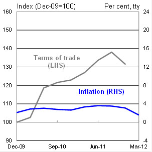
Source: ABS cat. no 5206.0, 6401.0 and Treasury.
This rise in the exchange rate acted as an important automatic stabiliser. While the high dollar weighed heavily on some sectors of the economy — as it continues to do so — it helped spread the benefits of the boom and shield the macro-economy from the shock by helping to bring down the price of imported consumer goods. The alternatives — tighter monetary policy or significant and costly increases in domestic prices (that is, a real exchange rate appreciation driven by higher domestic inflation) — would have a different distribution of costs on the economy, and ones which are arguably less beneficial for consumers.
In the absence of sound macroeconomic policy frameworks, past booms, such as the Korean War wool boom of the 1950s and the commodity boom of the early-1970s, ended badly.4 Annual inflation spiked at over 20 per cent in 1951-52, while in the 1970s annual inflation rates averaged just below 15 per cent for several years and unemployment rose.
One way to think about this is that, in these earlier booms, an external impulse, the terms of trade shock, fed directly into the economy through a fixed or only slowly adjusting exchange rate. This shock was then propagated throughout the economy via the centralised wage fixing system which led to considerable cost increases, and erosion of internal competitiveness, for those sectors not linked to mining.
In contrast, while the terms of trade boom during the first phase of the mining boom was larger than in either the 1950s or 1970s, the economy was first buffered by the floating exchange rate and then again by more flexible labour markets — so that for the first time in our history Australia was able to successfully manage the shock.
Shock 2 — the global financial crisis
Shock 2, the global financial crisis, was easily the most significant negative shock to strike Australia in the last 50 years.
Following the collapse of Lehman Brothers in the United States, the IMF repeatedly downgraded its growth forecasts for the advanced economies and the world. And by March 2009, the IMF was forecasting global GDP to decline by a ½ to 1 per cent in 2009 — the first time in history the IMF had forecast a global contraction.
Although Australia performed better than most advanced economies, the GFC still had a significant effect on the Australian economy. One of the most notable channels in Australia was financial asset prices.
Chart 6 gives a sense of the completely different scale of the domestic financial effects from the global financial crisis than from either the Asian financial crisis of the late 1990s or the dotcom bust of the early 2000s. Over the two years, 2007–08 and 2008–09, households suffered total capital losses equivalent to almost a full year's net disposable income. By contrast, neither the Asian financial crisis nor the dotcom bust resulted in any net capital loss for Australian households in aggregate.
Chart 6: Net saving plus capital gains and losses
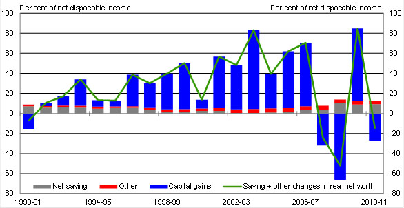
Source: ABS cat. no. 5204.0 and Treasury.
The shock hitting Australia during the GFC was remarkable, as was the speed and magnitude of the policy response. Indeed, it is the success of the policy response that feeds perceptions that there was no need for the policy response itself. The problem here, though, is that none of us can see directly what was avoided, although it doesn't take much effort to look abroad and see what could have eventuated here.
During those earlier events, monetary policy and the automatic stabilisers supported aggregate demand; discretionary fiscal policy was not required. This is because these shocks were — correctly — not seen to be either such extreme events or to precipitate circumstances where the effectiveness of monetary policy might be impeded.
The GFC was different. It was a much larger shock that arrived very quickly and, unlike many other shocks, came with a clear warning of its impending arrival — the Lehman Brothers collapse.5
As a result, Australia's macroeconomic policy, both monetary and fiscal policy, was able to move rapidly to support aggregate demand in a timely manner.
Almost every country in the world undertook macroeconomic stimulus to try and counteract the negative shock that had emanated from the United States. Indeed, monetary stimulus in the United States and the United Kingdom has pushed them close to the lower bound (i.e. into a liquidity trap with close to zero interest rates) and quantitative easing has been employed.
The Reserve Bank eased monetary policy significantly and swiftly in response to the global downturn. The cash rate was cut from 7.25 per cent at the start of September 2008 to 3 per cent by April 2009, a reduction of 425 basis points over seven Board meetings. Such was the speed of the Reserve Bank's response, 375 basis points of this easing occurred in the four Board meetings from October 2008, three weeks after Lehman Brothers collapsed, to February 2009.
In addition to the monetary policy response, fiscal policy was also used to support the economy. The Government used its balance sheet to support the effective operation of financial markets — for example, through guarantees for deposits and for wholesale debt securities — while also undertaking significant discretionary fiscal stimulus. Overall, the fiscal stimulus was forecast to increase GDP growth by 2 percentage points in 200
9 and to detract around 1 percentage point from growth in 2010.6 The automatic stabilisers also supported the weakening economy.
With a significant shock to the Australian economy leading to excess capacity, combined with a globally coordinated fiscal response to the crisis — limiting leakage through the exchange rate — fiscal stimulus was expected to provide substantial support to the domestic economy. I will come back to this issue shortly.
The size and the speed of monetary and fiscal policy response are also likely to have helped consumer and business confidence in the economy, further enhancing its effectiveness.7
Furthermore, the dollar fell by around 30 US cents, improving the competitiveness of our trade exposed industries and, again, acting as a partial shock absorber for the economy.
The rapid and significant response by monetary and fiscal policy, coupled with a well regulated financial system and strong growth in Asia meant that Australia came through the GFC relatively unscathed. However, there was still work to do once the worst of the crisis had abated.
Shock 3 — A renewed mining boom with GFC after-effects
With the recovery from the GFC, the economy entered a third phase, shock 3, which continues to this day, a phase some label ‘Mining Boom Mark II'.
While following the GFC, the terms of trade rebounded and reached a new record high, this has occurred against a backdrop of global uncertainty and more cautious households.
Once the recovery was under way, the task for both fiscal and monetary policy was to unwind the emergency levels of stimulus provided in response to the GFC.
In terms of its contribution to economic growth, fiscal stimulus peaked in the first half of 2009, and was progressively unwound from that point. By the March quarter 2010 fiscal stimulus was no longer contributing to growth.
Stimulatory monetary policy settings began to be wound back from October 2009. By May 2010 the cash rate had been increased sufficiently to return lending rates to around average levels.
With the perceived risk of inflationary pressures from an economy with limited spare capacity, a further modest tightening of monetary policy was deemed appropriate towards the end of 2010.
However, by the end of 2011 price pressures had abated and, with escalating concerns about the sovereign debt/balance-of-payments crisis in the Euro-zone, monetary policy was eased.
The recent further easing in monetary policy at the same time fiscal policy is consolidating has led a few commentators to argue that monetary and fiscal policy are now working in opposite directions. It is also argued that the fiscal consolidation in 2012-13 may take too much out of the economy.
I will address each of these in turn.
Before I do, let me make some general comments about the impact of discretionary fiscal policy on the macro-economy.
I have to admit that I am intrigued by the arguments put forward by a number of commentators on this issue. Obviously, it is not a new issue, with people arguing strenuously in recent years that the fiscal stimulus injected during the GFC had no impact on economic activity. For consistency, those same people presumably argue that that any fiscal consolidation must also have no impact on the macro-economy.
So let's consider the argument.
Typically it runs that in an open economy with a floating exchange rate and an inflation targeting central bank, an injection of fiscal stimulus is offset by an appreciation in the exchange rate and a decline in net exports, resulting in a multiplier of close to zero — this is standard Mundell-Fleming.
As my colleague David Gruen has noted previously — drawing on the 2010 work of the IMF and Ilzetzki, Mendoza and Vegh — this standard result seems broadly correct for countries with very high levels of public debt and where further fiscal loosening can result in a serious loss of confidence because of rising concerns over the solvency of the government.8 In that case, fiscal loosening will not stimulate domestic economic activity. This standard Mundell–Fleming result also appears to be broadly correct for countries with high trade shares.
But as David has also noted:
“for less open economies with low government debt like Australia, fiscal multipliers for temporary discretionary fiscal stimulus appear to be positive and sizeable.”
And, as noted earlier, we also know that coordinated fiscal expansion — of the sort pursued in the GFC — results in less leakage and hence larger multipliers.
As an aside, a clear example of the contractionary effects of discretionary fiscal tightening in a country with a floating exchange rate, an inflation targeting central bank and high, but far from unprecedented levels of government debt, is playing out in front of us at the moment. The United Kingdom has seen a notable stalling of its recovery from the GFC since the inception of its consolidation — a fiscal contraction of 2.8 per cent of GDP has coincided with near zero GDP growth in that time. Moreover, unlike the epicentre of the GFC, the USA, to say nothing of Australia, the UK still has a level of GDP some 4.3 per cent below its pre-GFC peak. In contrast, after the same period into the Great Depression, UK GDP was almost 1 per cent above its previous peak.
In short, the standard Mundell-Fleming theory appears to hold under a specific set of conditions, but when these conditions are relaxed discretionary fiscal policy has significant real effects, and to suggest otherwise risks a triumph of ideology over experience.
Now for Treasury to be consistent, we would have to assume that the fiscal consolidation announced in the Budget has a contractionary effect on activity, which indeed we have done.
However, it is not necessarily the case that one should expect the fiscal multipliers to be the same in the expansion and contraction phases.
Moreover, in a situation of close to full employment, the net effect of fiscal consolidation and a monetary easing would presumably be smaller than in a situation of either significantly under-utilised resources or where monetary and fiscal policy were both moving in the same direction.
So, back to the two questions.
Are fiscal and monetary policy working at cross purposes?
As I have already noted, the primary objective of fiscal policy, outside of extreme events like the GFC, is to maintain the budget in a sustainable position from a medium-term perspective, while monetary policy should play the primary role in managing demand to keep the economy stable.
In an economy with unemployment forecast to be not far from reasonable estimates of its lowest sustainable rate, and commodity prices remaining near historical highs, it is appropriate that the budget return to surplus to remain consistent with the medium-term fiscal objective.
So, rather than working at cross-purposes, the current directions of monetary and fiscal policy simply reflect a return to their normal roles following an extreme event.
Could fiscal consolidation take too much out of the economy?
The impact of fiscal consolidation on economic activity, whether discretionary changes or through the operation of the automatic stabilisers, is much more nuanced than implied by simply looking at the magnitude of the fiscal consolidation — around 3.1 per cent of GDP in 2012-13.
The impact of fiscal consolidation is a function of the size of the relevant fiscal multiplier — which depends on a number of factors
First, as mentioned earlier, fiscal multipliers are not and should not be expected to be constant over time. They will differ with economic circumstances. In an economy with a large amount of excess capacit
y, stimulus measures should have a larger impact on activity. In contrast, where the economy is close to full employment, the net effect can be expected to be much smaller as the exchange rate and monetary policy offset the fiscal stimulus.
With the economy not far from full capacity, multipliers associated with fiscal consolidation in Australia today are likely to be significantly lower than what they were for the discretionary stimulus provided during the GFC.
Second, in considering the economic impact of fiscal consolidation, it is important to consider both the types of decisions and the timing of their implementation. For example, a decision to reduce outlays in total but also to redistribute them in favour of those with high marginal propensities to consume would be less contractionary, and perhaps even stimulatory, than an across-the-board cut.
Equally, small shifts in the timing of outlays can influence the measured consolidation while leaving economic activity little affected. And where outlays which are predominantly spent overseas are reduced, the domestic impact is minimal.
It is also worth highlighting that to the extent there is weakness across the economy, monetary policy is well-placed to respond, unlike in many other advanced economies.
In fact, if subdued growth in the non–mining economy results in further increases in spare capacity, putting downward pressure on inflation, monetary policy is more likely to be an effective remedy as these sectors are typically more sensitive to interest rates and exchange rates.
The timing of fiscal consolidation
There are also those who argue that returning the budget to surplus in 2012-13 is a political gesture and there would be no great harm in delaying this by a year or so.
The problem with this argument is that if it's not appropriate to restore the structural budget position when we have low unemployment and the economy is expected to grow at around trend, when will it be appropriate?
It is surprisingly under–appreciated that fiscal consolidation in Australia is happening in a far healthier economic environment than the circumstances facing many other advanced economies at present.
Many of these economies are stuck between a rock and a hard place. Monetary policy is at or close to the lower bound; fiscal positions, which have long been in deficit, have been driven by the GFC to a situation with government debt reaching over 100 per cent of GDP in some cases. In this environment, traditional monetary policy is no longer effective and opportunities for fiscal policy are limited.
It is fortunate that Australia doesn't face the same wrenching predicament. But continued discipline is important to ensure we never get into this situation.
I have noted elsewhere that government at all levels face difficult fiscal circumstances for the foreseeable future, with razor thin surpluses at best in the absence of conscious decisions to raise additional revenue or cut outlays. 9
Efforts to reduce outlays are likely to be more effective, and sustainable, if nested within a broader assessment of the roles and responsibilities of the different levels of government, an approach that could help sharpen the focus on duplication, overlap and inefficiency. In this regard, the announcement at the recent COAG meeting that the Commonwealth and the States will work cooperatively to ensure that State environmental approval processes can satisfy Commonwealth obligations, reducing duplication and double handling, is a good initiative. However, even total success in minimising overlap will not address the key challenge — the gap between the expectations of government held by the Australian public and the public's willingness to pay what's required if those expectations are to be met.
With substantial risks remaining in the global economic environment, it is critical that we move now to recharge the fiscal batteries while circumstances remain favourable. By doing this, we will ensure that we retain the fiscal capacity to respond to future adverse shocks where needed as well as long-term trends such as those highlighted in the intergenerational reports.
Chart 7: Average OECD and Australian gross government debt since the 1970s
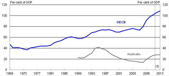
Note: Gross government debt refers to all levels of government.
Source: OECD Economic Outlook 90 database.
Across the OECD government debt ratios have steadily been on an upward trend since the 1970s. While there have been periods of governments reducing their debt–to–GDP ratios in good economic times, this reduction has been insufficient to stem the rise that follows in times of economic distress (Chart 7). This trend is even more concerning given that the effects of population ageing in most of these countries are still to be fully felt.
The good news from Australia's perspective is that we are not in the same boat, but we cannot assume this will always be the case.
Thank you.
1 The forecast error in export growth in 2010-11 was driven by a slower-than-expected recovery in Queensland coal exports in the March and June quarters of 2011 and ABS methodological changes to historical data. Revised assessments of the Australian coal industry supply chain after Budget 2011-12 identified capacity utilisation issues and expansion delays directly as a result of the 2011 floods, along with over-optimism in previous forecasts of timelines for new capacity coming online. These factors were also incorporated into our current forecasts.
2 Parkinson, M (2011), Sustainable Wellbeing — An Economic Future for Australia, The Shann Memorial Lecture, August 2011.
3 In assessing the stance of fiscal policy at the time, it is relevant to note that the economy was growing above trend, with unemployment falling, and with CGT and other revenues rising much faster than trend. While surpluses were also rising as a share of GDP, the fiscal settings were unlikely to have been optimal. However, the case for even tighter fiscal settings was made more difficult by the strength of the Government’s balance sheet and the approach to asset management.
4 Note that the mining investment boom of the late 1970s and early 1980s is excluded from this analysis as it was not driven by the terms of trade. Rather, that period was characterised by significant investment on the back of large resource discoveries even though the terms of trade had fallen after the early-1970s boom and had then remained broadly flat.
5 While the GFC significantly impeded global financial markets, it did not materially impede domestic monetary policy once bank borrowings were guaranteed by the Commonwealth government.
6 McDonald, T and Morling, S (2011), The Australian economy and the global downturn, Part 1: Reasons for resilience, Economic Roundup Issue 2, September 2011.
7 Gruen, D and Stephan, D (2010), Forecasting in the Eye of the Storm, Address to the NSW Economic Society, June 2010.
8 Gruen, D (2011), Lessons about Fiscal Policy from the 2000s, Comments at the 2011 RBA Annual Conference, published December 2011. See also IMF (2010), Will it
Hurt? Macroeconomic effects of Fiscal Consolidation, World Economic Outlook Chapter 3, October 2010; and Ilzetzki, E, Mendoza, EG, and Vegh, CA (2010), How Big (small?) are Fiscal Multipliers, NBER Working Paper 16479, October 2010.
9 Parkinson, M (2012), Introductory Remarks, Australia-Israel Chamber of Commerce, March 2012.