Budgeting in Challenging Times

Good afternoon. It is a pleasure to be here with you once again.

As you know, and has been much commented on of late, the past few years have been a challenging period for economic and revenue forecasting. Yet, despite considerable global volatility and structural changes domestically, the Budget forecasts for the volume of economic activity and employment - the real economy - have held up reasonably well over this period. The same cannot, however, be said of the forecasts of nominal GDP and tax revenue.

The direct impact of the, now well-known, overestimation in tax receipts is that the Australian Government faces a more difficult fiscal environment than had been anticipated a year ago.

Today, I want to take you through some of the drivers of recent weakness in nominal GDP growth and the Government's tax receipts, and consider why the extent of this weakness had not been anticipated. These drivers include:

• the difficulty that we, and other economic forecasters, have had in predicting the future path of global commodity prices, the exchange rate and capital gains; and
• the significant structural changes that have taken place since the Global Financial Crisis in the Australian economy and in the Government's tax base.

I will provide my assessment of the extent to which these drivers are likely to be permanent or temporary; take you through what we are doing to improve our forecasting processes; and conclude with a few brief points on the role that higher productivity could play in promoting the fiscal sustainability of all levels of government in Australia over the medium term.

Structural budget balances

Before turning to these topics though, I'll start with a few brief points about structural budget balances following the Treasurer's announcement this morning that he has commissioned us to produce updated estimates.

Estimates of the structural budget balance adjust for temporary factors that have a significant impact on the budget balance.

For the Australian Government, these factors include cycles in the real economy, and deviations in the terms of trade and capital gains tax receipts from their estimated long-run, or 'structural', levels.

Considered alongside underlying cash balance estimates and balance sheet indicators, structural budget balance estimates can provide guidance on whether current fiscal policy settings are sustainable over the medium term.

Structural budget balances are not difficult to produce, as is evident from the proliferation of think tanks and economic consultancies that are now producing structural budget balance estimates in Australia.

But as we have made clear before, there are significant caveats that are associated with this type of analysis, which can lead to problems of misinterpretation and misuse unless the reader is alerted to these.

In particular, identifying the structural or long run level of variables like the terms of trade and capital gains is conceptually challenging, with different assumptions for these variables leading to very different results.

Therefore, those that produce structural budget balance estimates should be transparent about their methodology, clear about their assumptions and open about how sensitive the estimates are to plausible changes in key parameters.

We will say more about these issues when we release our updated estimates of the structural budget balance for the Australian Government in the coming days.

Near-term economic outlook

Let me now move on to a brief summary of how we see the near-term outlook.

Against the backdrop of a still fragile global recovery, the Australian economy is expected to undergo two large and important transitions over the next few years. The first is in the resources sector, which is transitioning from the largest investment boom in our history to the 'production and exports phase'. 

While it will be significant in isolation, we do not expect the increase in resource production to be enough to offset the decline in resource investment. Accordingly, the net contribution of the resource sector to real GDP growth is expected to fall. Moreover, the production phase of the resource boom will also be significantly less labour-intensive than the investment phase.

This highlights the need for a second transition in the economy, to growth driven by the non-resource sectors.

This transition will be supported by low interest rates, but challenged by continued weakness in the global economy and a persistently high Australian dollar, even after the welcome falls in the past week.

Taken together, these factors lead us to forecast real GDP growth of around 2¾ per cent and 3 per cent in 2013-14 and 2014-15, or close to trend growth.

However, as the Treasurer has emphasised, there is a risk that these transitions will not be seamless - significant changes in the economy rarely are.

Still, with a low unemployment rate, well-contained inflation and low public debt, Australia embarks on this transition with some of the strongest economic fundamentals in the developed world.

Challenges in forecasting the nominal economy

Now, while the real economy has been growing at around its trend rate in recent years, it is the performance of the nominal economy that matters for government revenues.

As you know, real GDP measures the aggregate volume of production in the economy while nominal GDP captures both the quantity of production (that is, real GDP), as well as the prices received for that production.

Nominal GDP growth has been notably weaker than had been anticipated, with our forecasts for nominal GDP growth in 2012-13 revised from 5 per cent in last year's Budget down to 3¼ per cent in this year's.

Decomposing this 1¾ percentage point downward revision to the forecasts sees real GDP growth down by ¼ of a percentage point, with the remaining 1½ percentage point downgrade attributable to lower forecast growth in the GDP deflator.

In other words, while our forecasts for the real economy have held up reasonably well, the same can't be said of our price forecasts.

The relative accuracy of our forecasts for employment and wages growth has meant that our forecasts for income tax withholding - the largest source of Government revenue - have changed very little since last year's Budget.

However, we have been genuinely surprised by the weakness in prices over the past year, as captured at the broadest level by the downward revisions to our forecasts for the GDP deflator.

I want to pause on this point because it's important.

The fact is that we have always found forecasting nominal GDP and revenue to be more challenging than forecasting real activity, as hard as that is. And while there has always been a margin of error around the forecasts, I don't believe they have blown out.

The mean absolute percentage error in our nominal GDP forecasts over the past 20 years has been 1.6 percentage points. Since the beginning of the mining boom in 2003 - a period of dramatically outsized movements in the terms of trade - this mean absolute percentage error has been larger at 1.9 percentage points.¹ So, slightly larger than the implied 1¾ per cent forecasting error for last year's Budget.

What then, is behind the errors in the GDP deflator forecasts?

As I'll describe in more detail later, they reflect a sharper-than-anticipated fall in the US dollar prices of our commodity exports, the surprisingly persistent strength of the Australian dollar and weaker-than-anticipated growth in domestic prices since the 2012-13 Budget.

This has resulted in weaker company profits across all sectors of the economy.

The National Accounts measure of corporate profitability (GOS) has fallen in each of the past five quarters (t
o December 2012), by a cumulative total of 9.2 per cent.

This cumulative shortfall is not far short of the falls in corporate GOS during the GFC (10.2 per cent) and the early 1990s recession (11.2 per cent).

This is the first time in the history of the quarterly National Accounts (beginning in 1959) that corporate GOS has fallen in more than three consecutive quarters.

At the 2012-13 Budget, we were forecasting below-trend growth in corporate GOS.²  But as Chart 1 shows, the outcome has been much weaker still.

Chart 1: Corporate gross operating surplus

Through-the-year growth)

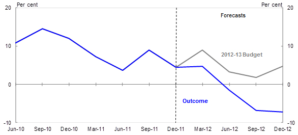
This weakness in corporate profits, combined with large shortfalls in year-to-date collections for capital gains tax and resource rent taxes, has resulted in large downward revisions to expected tax receipts in 2012-13 and over the forward estimates.

Note that the May 2012 Budget forecast growth in total tax receipts for 2012-13, of 10.8 per cent, on the back of a nominal GDP growth forecast of 5 per cent, was broadly similar to the experience of 2011-12, where actual growth in tax receipts was 10.4 per cent while growth in nominal GDP was 5 per cent.

However, as it has turned out, forecasts of tax receipts for 2012-13 have now been reduced by around $17 billion - $7.5 billion of that coming from company tax and $3.6 billion from capital gains tax. 

As a percentage of total tax receipts, this write-down is significantly greater than the downward revision to tax receipts in 1990-91, when Australia was last in recession, and is roughly two-thirds of the downward revision in 2008-09 at the onset of the global financial crisis.

Forecasting review

To be clear then, downward revisions of this magnitude are rare outside of major economic downturns.

Therefore, we have made it a priority to understand what has driven the revisions and to evaluate whether changes are required to our forecasting tools and procedures.

An important contribution to this process was the recent Review of Treasury's Economic and Revenue Forecasting Performance (the Review) - the third such review in the past two decades, following those in 1995 and 2005.

The 2012 Review examined Treasury's economic and tax revenue forecasting performance over the past 20 years, with a specific focus on the years leading up to, and since, the global financial crisis.

It was overseen by an independent external reference panel, chaired by Dr David Chessell (Chair of Access Capital Advisers) and comprising prominent private and public sector economists with a wealth of practical experience in forecasting.³

The Review was both thorough and extensive. It was a detailed and rigorous assessment of Treasury's forecasting performance against international best practice and the performance of other domestic forecasters, including the RBA, Deloitte-Access Economics and market economists.

The Review has been available on the Treasury web-site since February this year, but has clearly not been as widely read as I'd hoped; including, it would seem, by many of those who publicly comment with conviction about Treasury's recent forecasting performance.

As such, I will spend a few minutes running through some of the Review's key findings and how we are responding to the recommendations of the external reference group.

A good place to start is with the external panel's conclusion, which was that:

"Treasury approaches the forecasting task in a very professional manner and the forecasts it generates are broadly as accurate as those of both domestic forecasters and those generated by comparable agencies in countries with similar institutional arrangements as Australia."

While this sounds like a pass mark for us, we don't see it that way - our objective is to do better than this benchmark and, historically, we have.

The Review further found that Budget forecasts of nominal GDP growth and taxation revenues exhibit little evidence of statistical bias over the past two decades, with the average Budget forecast errors not significantly different from zero over this period.

However, the Review also found that, with the benefit of hindsight, Treasury has tended to underestimate growth in nominal GDP and taxation revenues during upswings and overestimate growth during downturns. To use the technical jargon, we have serially correlated errors.

The Review demonstrates this through case studies conducted over two discrete time periods: the years leading up to the GFC, a period referred to as 'Mining Boom Mark I'; and the period since the GFC. ⁴

As many of you may recall, prior to the GFC, Treasury was criticised for consistently underestimating growth in nominal GDP and tax receipts, primarily due to a consistent pattern of underestimating growth in the terms of trade.⁵

Since 2005-06, we have been projecting declines in the terms of trade, reflecting an expectation that the global supply response to high non-rural commodity prices would start to outpace growth in demand from emerging Asia.

This view was based on extensive analysis and discussion, including with the mining sector.⁶ 

However, like the sector itself, we consistently underestimated the strength of growth in emerging Asia and consistently overestimated the pace at which new global supply would be brought on-line.

The result was that the terms of trade and nominal GDP growth continually surprised on the upside.

The recent Review also finds that Treasury consistently underestimated taxation revenue over this period. This can be explained, at least in part, by our underestimation of commodity prices and nominal GDP growth.

Another source of underestimation bias during the Mining Boom Mk I was capital gains, which also consistently surprised on the upside.

The 2005 Review catalysed a major overhaul of the models and improvements in the quality of data sets that we use to forecast tax receipts.

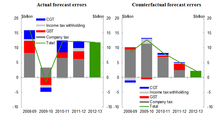
To judge the success of these changes, the 2012 Review contains a counterfactual exercise that compares the actual revenue forecasting errors during Mining Boom Mk I to those that would have occurred if our forecasts for nominal GDP and asset prices were correct. The results are shown in Chart 2.

Chart 2: Contribution to Budget taxation revenue forecast error by major head of revenue

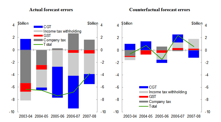
Note: Total error is the sum of revenue heads shown, and not the error for total tax receipts. The counterfactual exercise uses as more refined model for forecasting CGT receipts than was available at the start of Mining Boom Mk I. This model was implemented from 2006-07, following a review of the CGT forecasting framework, which was undertaken due to the large error in forecasting CGT receipts in 2005-06.

On the basis of the counterfactual exercise, the Review finds that most of the revenue forecasting errors during the latter stages of Mining Boom Mk I are attributable to errors in our forecasts of the nominal economy and asset prices, rather than any systematic tendency to underestimate revenue during a boom period.

This show
s that the changes to our revenue forecasting models that were made in response to the 2005 Review were successful in significantly reducing one source of error in our revenue forecasts - those attributable to weaknesses in the revenue models themselves.

It also highlights another important finding of the recent Review, which was that:

"Treasury's forecasting methodology operates in an environment of continuous internal evaluation and development, with forecast errors regularly reviewed, driving a quest for improvements in forecasting practices."

The changes that we are making in response to the recent period of overestimation - and our progress in responding to the recommendations of the most recent Review - serve as further evidence of the strength of our commitment to continuous improvement. 

Treasury's forecasting performance

Before I elaborate on this, though, I will put the recommendations of the recent Review in context by describing the factors that have driven our forecasting errors since the GFC.

In doing so, I'll focus on the changes to our forecasts since the 2010 Pre-Election Economic and Fiscal Outlook (or PEFO) - a period in which nominal GDP growth and taxation revenue have been consistently overestimated.

The forecasting challenges that we have confronted recently are best understood in the context of the enormous structural changes that have taken place in the economy and tax base over the past few years.

While some of these structural changes were discussed in previous Budget updates, the magnitude of the impacts was underestimated. The result has been a succession of forecast downgrades, including since last year's Budget.

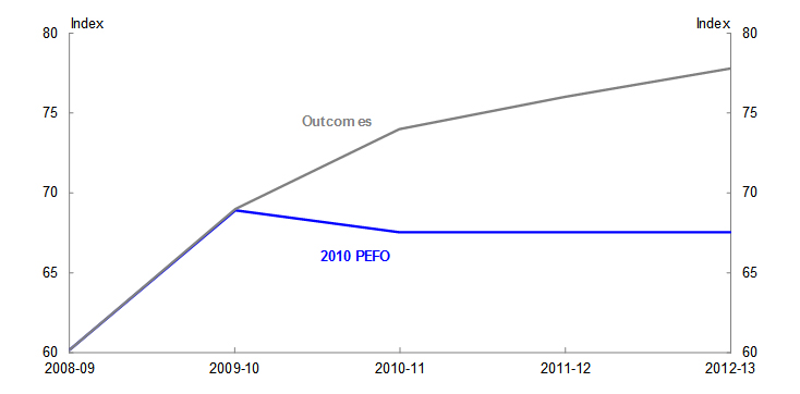
Let's start with nominal GDP. As shown in Chart 3, the level of nominal GDP to 2012-13 relative to our baseline in 2008-09 is now forecast to be more than 4 percentage points lower than projected at the 2010 PEFO.⁷

This means that, in 2012-13, nominal GDP will be around $53 billion below our projection at the 2010 PEFO.

Chart 3: Nominal and real GDP forecast performance

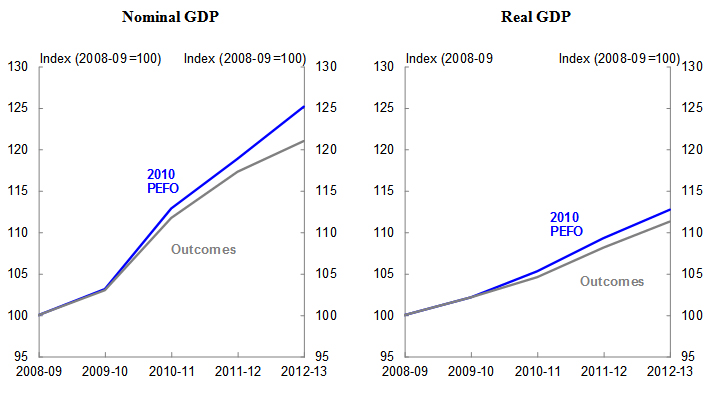
Note: At 2010 PEFO, 2009-10 to 2011-12 were forecasts and 2012-13 was a projection. The outcome for 2012-13 is the estimate at the 2013-14 Budget.

If we decompose this we find that growth in real GDP to 2012-13 is now forecast to be 1.4 percentage points lower, or around one-third of the implied forecast error for nominal GDP growth.

So, consistent with the explanation that I gave earlier, the main driver of the downward revision to our forecasts for growth in nominal GDP is weaker-than-anticipated growth in the GDP deflator.

The deflator represents the prices of goods and services that we produce, including both the products that are purchased domestically and those that are sold as exports. Thus, the GDP deflator has two elements: export prices and domestic prices.

Let's look at these in turn, starting with domestic prices. We measure these prices using the deflator for Gross National Expenditure (GNE) less import prices.⁸

Chart 4: Domestic and export prices

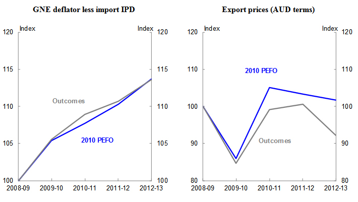
Note:  At 2010 PEFO, 2009-10 to 2011-12 were forecasts and 2012-13 was a projection. The outcome for 2012-13 is the estimate at the 2013-14 Budget.

Our forecast for the level of the GNE deflator less import prices in 2012-13 has held up well. I'm not claiming that we were blessed with perfect foresight for this particular forecast. The point is just that, looking over the past several years, this isn't the source of our forecast revisions.

Rather, the key driver is export prices. It's not that we didn't expect export prices to fall - indeed, we have been factoring in price falls since 2005-06. At the 2010 PEFO, we forecast that they would start falling from 2010-11.

When they did start to fall, they fell much more sharply than we forecast. This possibility had been noted at the time - page two of the 2010 PEFO stated that:

There are substantial risks around the future profile of the terms of trade, with considerable short-term volatility in spot commodity prices and uncertainty about the timing, pace and extent of their decline as increased global supply capacity comes on line.

The more sudden and steep decline that actually occurred meant that our export price forecasts for 2012-13 measured in Australian dollars are almost 10 percentage points lower now than projected in the 2010 PEFO.

When thinking about movements in export prices in Australian dollar terms, it is helpful to think about both changes in the foreign currency price and the exchange rate.

Typically, a fall in export prices and Australia's terms of trade would coincide with a fall in our exchange rate. Thus, we would expect that the impact on national income of a decline in export prices would be partly offset by a depreciation of the exchange rate, therefore providing a buffer to the fall in profits across the traded sector.

This is where something out of the ordinary has occurred. The Australian dollar is around 15 per cent higher in trade-weighted terms than we were assuming at the time of the 2010 PEFO (Chart 5), which more than explains the forecast error in export prices.⁹

Chart 5: Trade Weighted Index

Note:  At 2010 PEFO, 2009-10 to 2011-12 were forecasts and 2012-13 was a projection. The outcome for 2012-13 is the estimate at the 2013-14 Budget.

The direct effect on export prices is likely to understate the contribution of the high exchange rate to our nominal GDP forecasting error, because the exchange rate appreciation has also made imports more attractive and competitive conditions, and hence profitability, more difficult for our trade-exposed manufacturing and services sectors, thereby also contributing to the downward revision to our forecasts for real GDP growth since the 2010 PEFO.

Chart 6 highlights the recent break down in the relationship between the terms of trade and our exchange rate. This relationship broadly held during the significant increase in the terms of trade from 2003-04 through to 2007-08, and even during the period of marked volatility associated with the global financial crisis. Where the relationship has fallen down is since the peak of Australia's terms of trade in the September quarter of 2011. Since then, the terms of trade has fallen 17 per cent, while the exchange rate has barely budged - at least until the past ten days.

Chart 6: Terms of Trade and the Trade Weighted Index

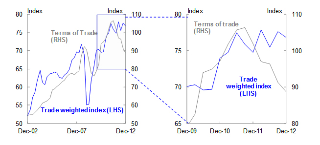
There have been periods in the past when factors other than the terms of trade have been more or less important in driving the exchange rate. And with the benefit of hindsight, it's easy to point to interest rate differentials and our relative attractiveness as an investment destination at a time of significant growth in global liquidity as factors that are supporting the current level of the exchange rate. My point is that the break-down in the relationship between the terms of trade and the exchange rate over the
past 18 months is not something that we could have predicted at the time of the 2010 PEFO.

Again, this is a point worth pausing on.

Forecasting movements in the nominal exchange rate is almost impossible. Along with the RBA, we have long been of the view that macroeconomic forecasts should be based on the technical assumption of no change in the exchange rate over the forecast horizon. But when the terms of trade fall by significantly more than expected, it is still a significant anomaly for the exchange rate to remain essentially unmoved.

It won't be lost on most of you I'm sure that the Australian dollar has depreciated over the past week, with the TWI now around 4 per cent lower than assumed for last week's Budget. While welcome, this demonstrates my point, which is that the nominal exchange rate can change significantly over short periods of time and sometimes with no apparent link to a change in fundamentals. In these circumstances, we believe that the best approach is to assume that the exchange rate won't change from its recent average, but highlight future movements as a risk.

At the time of the 2012-13 Budget, our forecasts were for the terms of trade to be 2¾ per cent lower in 2012-13 than in 2010-11. Our latest forecasts are for the decline over this period to be 7 per cent, or over 4 percentage points greater.¹⁰

Notwithstanding this, the assumption in this Budget for the trade weighted exchange rate based on the recent average is actually slightly higher than that used in last year's budget - again, highlighting the recent break down in the historical relationship.

So, how does this hit tax revenue?

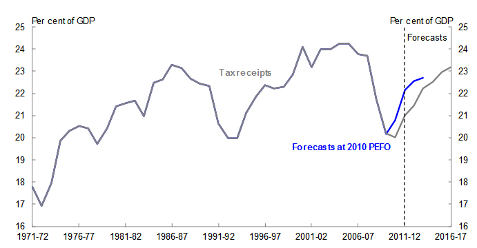
Weaker-than-anticipated growth in nominal GDP has contributed to a large downward revision to forecast tax receipts. At the 2010 PEFO, we were projecting tax receipts to be $354 billion in 2012-13, some $28 billion higher than the forecasts presented in last week's Budget.

Chart 7: Tax receipts

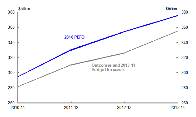
Note: At 2010 PEFO, 2009-10 to 2011-12 were forecasts and 2012-13 was a projection. The outcome for 2012-13 is the estimate at the 2013-14 Budget.

However, in contrast to the counterfactual that I showed for Mining Boom Mk I - where our revenue forecasting errors in the period immediately preceding the GFC were almost entirely attributable to our economic forecasting errors - other forces have also affected the tax take since the GFC.

The downward revision to tax receipts in recent years is also due, in part, to a lower revenue yield per dollar of GDP. From its pre-crisis level of 23.7 per cent in 2007-08, the tax-to-GDP ratio fell 3.6 percentage points to 20.1 per cent in 2010-11, the biggest decline in the ratio since the 1950s.

This reflects both the successive large cuts to personal income tax rates implemented between 2005-06 and 2009-10 and a fundamental change in the relationship between the nominal economy and tax receipts.

One way to demonstrate this change in the relationship between the economic aggregates and tax revenues since the GFC is to replicate the counterfactual that I showed earlier.

Using the same approach, Chart 8 compares the actual revenue forecasting errors since the GFC to those that would have occurred if our forecasts for nominal GDP and asset prices had been correct.

Chart 8: Contribution to Budget taxation revenue forecast error by major head of revenue

Note: Total error is the sum of revenue heads shown, and not the error for total tax receipts. The forecast errors shown for 2012-13 are calculated based on the forecasts at the 2013-14 Budget, produced using the new three-sector company tax model described below. The change in forecast tax receipts in 2012-13 is not disaggregated as large movements between tax heads in the final two months of the financial year can give a misleading picture of forecast errors.

What this counterfactual shows is that the errors for most revenue heads are reduced significantly if we use actual economic outcomes rather than forecasts.

However, in contrast to the Mining Boom Mk I counterfactual, there are significant residual errors for the company tax revenue head. While these errors have fallen over time, they remain large.

Until recently, the model that we were using to forecast company tax receipts was for the whole corporate sector. The 2012 Review found that this whole-of-economy model was not well-suited to cases where sectors of the economy are growing at very different rates, as has been the case since the GFC.

There are two reasons for this.

The first is that the whole-of-economy company tax forecasting model does not distinguish between the characteristics of different sectors, such as the capital intensive nature of the resource sector and its lower effective company income tax rate.

Since 2008-09, the ratio of company tax paid to net operating surplus (NOS - GOS adjusted for depreciation) for resource companies has been around 5 to 10 percentage points less than for the corporate sector as a whole.

Just to be clear, this is not a judgement about what the effective tax rate paid by mining companies should be - it is simply a statement of fact.

The relatively low effective tax rate paid by resource companies reflects a range of factors, including royalty deductions, the capital-intensive nature of mining and the accelerated rates at which investment - especially in the oil and gas sectors - can be written off for tax purposes.

Increasing levels of investment in this sector have seen annual mining depreciation growth triple, from around 4.5 per cent in 2003-04 to 15 per cent by 2011-12, weighing on the government's tax take.

High prices for resource exports have also boosted resource sector profits so much that mining's share of corporate gross operating profits has doubled since 2003-04. By contrast, the financial sector's share of company tax payments is roughly a third of what it was prior to the GFC.

The mining sector's low effective tax-to-NOS ratio means that an increased share of mining profits in total profits and nominal GDP has lowered the tax-to-GDP ratio.

Therefore, a significant driver of the weaker-than-expected outcomes for company tax has been both the rising share of mining profits in total GOS and stronger-than-expected growth in depreciation deductions resulting from the resource investment boom.

The second factor identified in the recent review as a contributor to the overestimation of company tax revenue since the GFC is that our previous whole-of-economy company tax forecasting model did not take sufficient account of companies operating on non-June accounting periods.

This includes the large financial companies that operate on an accounting year ending in September and the large resource companies whose accounting year ends in December, making it more difficult to accurately estimate the timing of the receipt of cash payments of corporate tax on underlying corporate profits (though not profitability in total).

In response, we have recently developed a three sector company tax model that splits the economy into mining, finance and insurance, and other sectors, and takes better account of the different payment patterns of companies that operate on non-June accounting years.¹¹

Another key reason the tax-to-GDP ratio has been unusually low recently is lower capital gains tax (CGT) revenue. CGT receipts were unusually high in the year
s leading up to the GFC, as strong growth in asset prices led to high levels of realised capital gains.

The decline in global share prices during the GFC, along with weak asset price growth since, has reduced CGT revenue to less than one-third of these peak levels as a share of GDP.

In addition to the challenge of predicting the future path of asset prices¹², the capital losses accumulated since the GFC have been larger and more persistent than we had appreciated, explaining the significant divergence between changes in equity prices and CGT receipts since the middle of 2009 evident in Chart 9.

Chart 9: Capital Gains Tax Receipts and Equity Prices

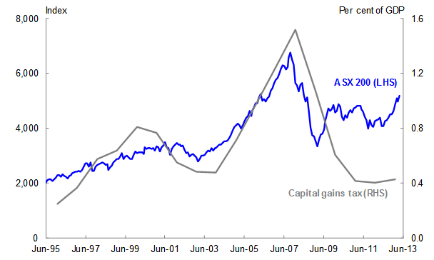
While CGT receipts are expected to recover somewhat over the forward estimates, they are not expected to return to pre-GFC levels, which reflected a period of strong asset price growth that is unlikely to be repeated in the foreseeable future.

This brings me to another of the recommendations from the recent Review - that we examine whether we can improve the accuracy of the technical assumptions for equity and housing prices that are used to generate the CGT revenue forecasts.

With the benefit of hindsight, one could ask why we didn't make the changes to our company tax and CGT modelling approaches sooner.

Forecasting during these periods of significant change, and recognising the fundamental shifts that are occurring in the economy and tax base, is extremely challenging in real time, something that we, our counterparts overseas and private sector forecasters have experienced in recent years.

Having said that, we recognise that - unlike private sector forecasters - our forecasts have significant implications for Government policy and hence the wellbeing of the Australian people.

With the stakes high, we strive to be the best - such that being on par with others does not detract from our determination that we can and should do better.

As such, I am committed to following through on all of the Review's recommendations.

In addition to what I have mentioned already, our response to one of the Forecasting Review's recommendations - that we should include in the Budget papers a high level review of the economic forecast errors (nominal and real GDP) for the previous financial year - can be found in last week's budget at Appendix A of Budget Statement 2. This complements the existing discussion of our revenue forecasting errors in Appendix D of Budget Statement 5. 

Before leaving the topic of forecasting, I want to touch briefly on the question of whether we should be publishing a range of economic and revenue forecasts.

All forecasts have notional "confidence intervals" around them - ranges within which different outcomes are all reasonably plausible. Indeed, the forecasting review provides data on the historical errors, in real GDP, nominal GDP and revenue.

Confidence intervals could be produced, on an ongoing basis, for real GDP, and also for forecasts of prices and hence nominal GDP. These nominal GDP confidence intervals would then reflect two sources of uncertainty - the outlook for real GDP and the outlook for prices.

There is also uncertainty in translating nominal GDP into revenue. As a result, confidence intervals around the revenue forecasts would compound three sources of uncertainty - real GDP, prices and the relationship between nominal GDP and tax revenue. While the bands might be quite wide, this could still aid understanding of the inherent uncertainties in the point estimates.

Medium-term fiscal outlook

Thus far I have focused on explaining the reasons behind the large downward revisions to our forecasts of nominal GDP and the government's tax receipts in recent years and the changes that we are making to our forecasting tools in response.

Some of the factors that are weighing on tax receipts are likely to be temporary.  For example, CGT losses incurred during the GFC will eventually wash out of the tax system, although this is taking longer than we had expected. Similarly, the impact of depreciation deductions is likely to decline as mining investment peaks.

The effect of lower nominal GDP levels, however, will be more long-lived. Let me explain.

In broad terms, outside of major economic downturns that undermine the productive capacity of the economy (so-called 'hysteresis effects'), the real economy is self-correcting: a period of below-trend growth is typically followed by a period of above-trend growth as the economy returns to full employment.

The same need not apply to nominal GDP - following a period of below-average growth, there is no reason to expect the GDP deflator to record above-average growth in coming years.

Consequently, while we have forecast that the tax take per dollar of GDP will return to levels broadly consistent with the long-term average over the forward estimates period, we expect the level of tax revenues in dollar terms to remain significantly below what we were forecasting at last year's Budget and MYEFO.

Chart 10: Tax-to-GDP Ratio

Another factor that will affect future revenue collections is the revision to the carbon price projections. The 2013-14 Budget projects a carbon price of $12.10 in 2015-16.

This change, along with updated emissions, means that compared with the 2012-13 MYEFO, receipts from the sale of carbon permits will be $3.7 billion lower over the four years to 2015-16. Partly offsetting this, expenditure on several programs in the Clean Energy Future plan will also fall because of decisions announced by the Government in last week's Budget.

The previous projections were based on the Strong growth, low pollution report published in 2011, which is a comprehensive modelling exercise underpinned by longer-term fundamentals such as the long-term global environmental goals. These fundamentals haven't changed. As such, the modelled prices continue to show the price levels required over time to meet these long-term goals as well as the international commitments to reduce emissions by 2020.

However, in the near term, the profound economic weakness in Europe has weighed heavily on the European carbon market. As the Australian carbon pricing mechanism will be linking to the European ETS from 2015-16, downward revisions to price projections largely reflect this weakness. This fall in the carbon price will mean that it will be cheaper for the Australian economy to achieve its emissions reduction target.

In summary, the medium-term revenue picture is this. Some of the current factors weighing on tax collections will fade with time and the impact of the lower carbon price will be muted by reduced expenditure.

As a result, the tax-to-GDP ratio should return to more normal levels although, as illustrated in Chart 10, we expect it will do so a couple of years later than previously anticipated.

More troubling, though, is that the impact of lower nominal GDP will be more long-lived, resulting in lower estimates of revenue collections across the forward estimates and beyond.

That is, while the tax collected from nominal GDP will return to its long-run share, the level of nominal GDP is likely to be permanently lower than we were projecting, meaning the dollar value of tax receipts will be lower than previously thought.

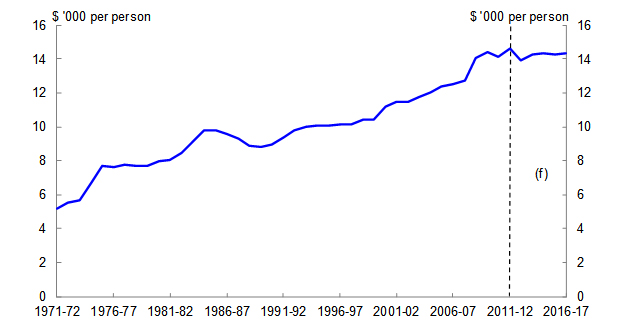
Let me turn now to the expenditure side of the budget. Since the beginning of the 1970s, real expenditure per person has almost tripled, increasing at a compound annual growth rate of 2.6 per cent (Chart 11).

Chart 11: Real government payments per person

Looked at in another way, the ratio of expenditure to GDP has generally remained fairly close to its average over the past 30 years (Chart 12).

Chart 12: Receipts and payments as a share of GDP

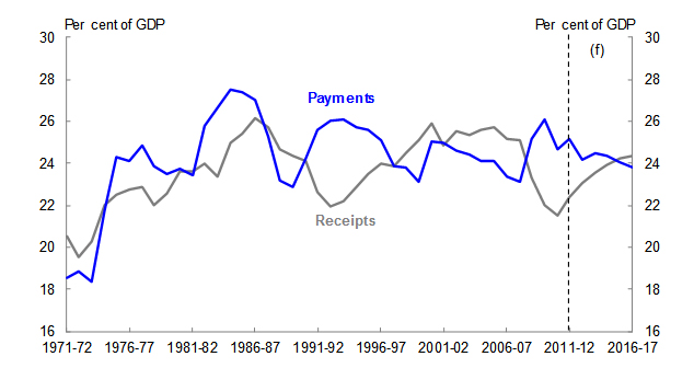
What this tells us is that, as the economy expands, government expenditure has tended to expand with it and thus the scope of government services per person has increased, albeit remaining roughly constant as a share of GDP.

We also know that health and pension expenditure are set to increase further as the population ages and as changes in preferences and technology drive increased expenditure on health services.

The confluence of lower nominal GDP levels leading to weaker-than-anticipated tax collections, demographic change, rising health and aged care costs and external risks all point to the challenge of maintaining fiscal sustainability over the medium term.

The link to productivity

This challenge could be alleviated, at least in part, by a sustained improvement in Australia's productivity growth performance.

As I've noted on previous occasions, improved productivity growth will be important in the next decade to help maintain growth in national income in the face of downward pressure from falls in the terms of trade and the ageing of the population.

Productivity-enhancing reforms will also be needed to ensure that Australia benefits from the next phase of the Asian century, driven by the demand for high-quality goods and services from an expanding Asian middle class.

Unlike the initial resources phase, Australia will need to compete with the likes of the US, Japan and Europe, and China and India themselves, on the basis of cost and quality, where our ability to do this will depend on how successful we are in raising productivity.

As I mentioned, there is another reason for pursuing productivity growth that links to my earlier points on the medium-term fiscal challenge, which is that productivity reforms can be a win-win from a fiscal perspective.

Policies directed at promoting market-based incentives, for example, tend not to entail substantial fiscal costs. At the same time, they help to expand the size of the economy and thus government revenues without generating inflationary pressures¹³.

Governments can also contribute to productivity growth more directly by enhancing the efficiency of public provision. This could occur, for example, through increased incentives for innovation in service delivery, or budget systems that reward efficiency and improvements whilst setting clear expectations. This is worth pursuing even if, for measurement reasons, the gains aren't captured in the productivity statistics.

Therefore, it is important that as we consider the fiscal challenges that lie ahead, we consider the role that an improvement in Australia's productivity performance could play in alleviating some of the pressures.

Conclusion

To conclude, the past decade has been a tumultuous period for the Australian economy, defined by some of the largest shocks - both positive and negative - in living memory.

We have: seen Australia's terms of trade rise to record highs; witnessed the largest downturn in the global economy since the Great Depression; experienced sharp rises and falls in asset prices; seen resource investment reach unprecedented highs as a share of GDP; been living through an unprecedented expansion in the importance of the mining sector as it has grown from around 5 per cent of GDP to 10 per cent in a decade; and watched as the exchange rate has appreciated to levels that we haven't seen in 30 years.

In these circumstances, we in Treasury have struggled to keep pace, with large revisions to our economic and revenue forecasts the result.

Our response has been to undertake a comprehensive review of forecasts overseen by an external panel. The Review highlighted some positives, but also recommended areas where we can improve.

Some of these recommendations have already been acted on in full and those that haven't are well in hand. The result is continued improvement in the methodological underpinnings of Treasury's forecasts.

Looking forward, some of the factors that have contributed to weaker-than-anticipated tax receipts are expected to persist, including the downward shift in the level of nominal GDP compared to what we had been anticipating.

Combined with growing community expectations of the role of government and rising costs associated with healthcare and the ageing of the population, this creates a challenging environment for fiscal policy in the years ahead - not only for the Commonwealth Government, but for state and local governments as well.

This challenge could be alleviated, at least in part, by an improvement in Australia's productivity growth performance, where policies that promote market-based incentives and/or succeed in enhancing the efficiency of government service provision can be a win-win for the fiscal position.

Thank you.